Credit risk
See also: Insurance and finance risk analysis modeling introduction, Credit ratings and Markov Chain models
Credit risk is the risk of loss due to a debtor's failure or partial failure to repay a loan or other credit instrument (bonds). We need three components to assess the credit risk of an individual obligor:
-
Default probability
-
Exposure distribution
-
Loss given default as a fraction of the exposure
Components 2 and 3 can sometimes be replaced by a single distribution of loss give default.
This topic describes how to fit probability distributions to data which are used to estimate 2 and 3 above. We can also estimate the binomial probability needed for the probability of default. There are a number of methods we can use to determine the aggregate distribution.
Single portfolio example
The figure below shows a credit risk model for a single portfolio of independent, Lognormally distributed random individual loss distributions where there are 2 135 debtors each with the same 8.3% probability of default.

Example model ![]() Credit_risk_single_portfolio - modeling credit risk for a single portfolio
Credit_risk_single_portfolio - modeling credit risk for a single portfolio
In this model the VoseAggregateMC function in Cell C11 is randomly sampling n Lognormal(55,12) distributions and summing them together, where n is itself a Binomial(2135, 8.3%) distribution. This is the 'brute force' Monte Carlo approach to summing random variables, but with the advantage that the simulation is all done within C++ (which is faster) and the final random sum returned back to Excel.
Since the model of the figure above is estimating a distribution of loss, the Value at Risk at the 95th confidence level is simply the 95th percentile of the output distribution, which is returned directly into the spreadsheet at Cell E11 at the end of a simulation. In this example, running 1 000 000 iterations produces a VaR of 10 943.62. We can take a different approach by constructing the aggregate distribution using Fast Fourier Transforms (using VoseAggregateFFT). Cell C13 generates random values from this distribution, whilst Cell E13 employs the U parameter to return the 95th percentile of the aggregate distribution directly without any simulation. The ModelRisk screen capture shown below shows this second use of the function.
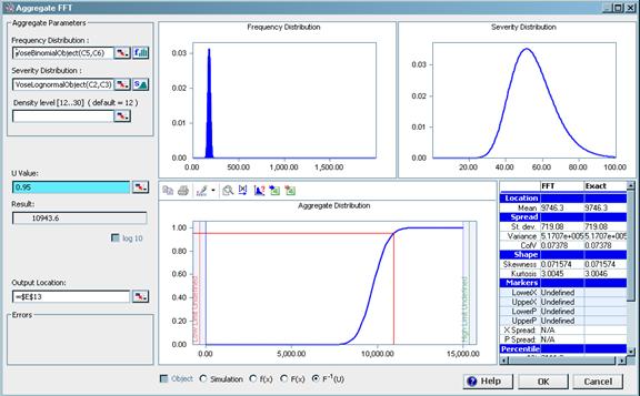
The Aggregate FFT window - directly calculating a percentile of the aggregate distribution
In Cell G13 the formula:
=VoseIntegrate("#*VoseAggregateFFTProb(#,C7,C4,,0)",E13,15000,1)
calculates the integral to determine the Expected Shortfall:

where E13 is the defined threshold, x is the value of the aggregate loss distribution, f(x) is the density function for the aggregate loss distribution (determined by the function VoseAggregateFFTProb( ...) ), and 15 000 is a sufficiently large value to be used as a maximum for the integral, as shown in the screen capture below:
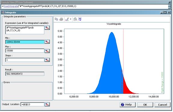
The ModelRisk Integrate window to determine the Expected Shortfall of a credit portfolio. The Steps parameter is an optional integer used to determine how many sub-intervals are made within each interval approximation as the function iterates to optimized precision.
Single portfolio example with separate exposure and loss given default distributions
In the beginning of this section I pointed out that one may generally have separate distributions for the amount of exposure a debt holder has, and the fraction of that exposure that is realised as a loss. This means that we need to determine the sum:

This is easily done with Monte Carlo simulation in a manner similar to the model of shown before but replacing the Lognormal variable with the product of two variables. Alternatively, with ModelRisk you can use the VoseSumProduct function to return the aggregate distribution with one cell formula. Both methods are shown in the example model below:

Example model ![]() Credit_risk_separated - Credit risk model with separate exposure and loss fraction components
Credit_risk_separated - Credit risk model with separate exposure and loss fraction components
The VoseSimulate function simply generates random values from its object distribution parameter, which allows the user to keep the distribution in one place in the spreadsheet rather than many. The VoseSumProduct(n,a,b,c...) adds n variables together where each variable is a*b*c*... where a,b,c, etc are distribution objects.
We can also construct the density function fL(x) for the individual loss distribution as follows:

where fF( ) is the density function for the loss fraction distribution and fE( ) is the density function for the exposure distribution. Then the loss given default distribution can be constructed and used in a FFT calculation. The ModelRisk function VoseAggregateProduct performs this routine, so we can write:
=VoseAggregateProduct(VosePoisonObject(1000), VoseLognormalObject(100,10), VoseBetaObject(11,35))
Default probability as a variable
Default probabilities can perhaps be considered constant over a short period, but over a longer period or where the market is very volatile it should also be modelled as a function of the condition of the economy and, for corporate credit risk, as a function of the state of the regional business sector too. The same may apply for the loss given default variable as the debt holder may recover a smaller fraction of the exposure in more stressing times. This means that we must construct credit portfolios that are disaggregated at an appropriate level and sum their cash flows. Failure to model these correlations will underestimate the risk of losses. For example, we might produce a model that varies the probability of default (PD) as a function of changes in GDP growth (GDP), interest rate (IR) and inflation (I) using an equation of the form:
PDt = PD0*Exp[Normal(1+a*(GDPt-GDP0)+b*(IRt-IR0)-c*(It-I0),s)]
where a, b and c are constants, t is some time in the future, s is a residual volatility and X0 means the value of the variable X now.
Navigation
- Risk management
- Risk management introduction
- What are risks and opportunities?
- Planning a risk analysis
- Clearly stating risk management questions
- Evaluating risk management options
- Introduction to risk analysis
- The quality of a risk analysis
- Using risk analysis to make better decisions
- Explaining a models assumptions
- Statistical descriptions of model outputs
- Simulation Statistical Results
- Preparing a risk analysis report
- Graphical descriptions of model outputs
- Presenting and using results introduction
- Statistical descriptions of model results
- Mean deviation (MD)
- Range
- Semi-variance and semi-standard deviation
- Kurtosis (K)
- Mean
- Skewness (S)
- Conditional mean
- Custom simulation statistics table
- Mode
- Cumulative percentiles
- Median
- Relative positioning of mode median and mean
- Variance
- Standard deviation
- Inter-percentile range
- Normalized measures of spread - the CofV
- Graphical descriptionss of model results
- Showing probability ranges
- Overlaying histogram plots
- Scatter plots
- Effect of varying number of bars
- Sturges rule
- Relationship between cdf and density (histogram) plots
- Difficulty of interpreting the vertical scale
- Stochastic dominance tests
- Risk-return plots
- Second order cumulative probability plot
- Ascending and descending cumulative plots
- Tornado plot
- Box Plot
- Cumulative distribution function (cdf)
- Probability density function (pdf)
- Crude sensitivity analysis for identifying important input distributions
- Pareto Plot
- Trend plot
- Probability mass function (pmf)
- Overlaying cdf plots
- Cumulative Plot
- Simulation data table
- Statistics table
- Histogram Plot
- Spider plot
- Determining the width of histogram bars
- Plotting a variable with discrete and continuous elements
- Smoothing a histogram plot
- Risk analysis modeling techniques
- Monte Carlo simulation
- Monte Carlo simulation introduction
- Monte Carlo simulation in ModelRisk
- Filtering simulation results
- Output/Input Window
- Simulation Progress control
- Running multiple simulations
- Random number generation in ModelRisk
- Random sampling from input distributions
- How many Monte Carlo samples are enough?
- Probability distributions
- Distributions introduction
- Probability calculations in ModelRisk
- Selecting the appropriate distributions for your model
- List of distributions by category
- Distribution functions and the U parameter
- Univariate continuous distributions
- Beta distribution
- Beta Subjective distribution
- Four-parameter Beta distribution
- Bradford distribution
- Burr distribution
- Cauchy distribution
- Chi distribution
- Chi Squared distribution
- Continuous distributions introduction
- Continuous fitted distribution
- Cumulative ascending distribution
- Cumulative descending distribution
- Dagum distribution
- Erlang distribution
- Error distribution
- Error function distribution
- Exponential distribution
- Exponential family of distributions
- Extreme Value Minimum distribution
- Extreme Value Maximum distribution
- F distribution
- Fatigue Life distribution
- Gamma distribution
- Generalized Extreme Value distribution
- Generalized Logistic distribution
- Generalized Trapezoid Uniform (GTU) distribution
- Histogram distribution
- Hyperbolic-Secant distribution
- Inverse Gaussian distribution
- Johnson Bounded distribution
- Johnson Unbounded distribution
- Kernel Continuous Unbounded distribution
- Kumaraswamy distribution
- Kumaraswamy Four-parameter distribution
- Laplace distribution
- Levy distribution
- Lifetime Two-Parameter distribution
- Lifetime Three-Parameter distribution
- Lifetime Exponential distribution
- LogGamma distribution
- Logistic distribution
- LogLaplace distribution
- LogLogistic distribution
- LogLogistic Alternative parameter distribution
- LogNormal distribution
- LogNormal Alternative-parameter distribution
- LogNormal base B distribution
- LogNormal base E distribution
- LogTriangle distribution
- LogUniform distribution
- Noncentral Chi squared distribution
- Noncentral F distribution
- Normal distribution
- Normal distribution with alternative parameters
- Maxwell distribution
- Normal Mix distribution
- Relative distribution
- Ogive distribution
- Pareto (first kind) distribution
- Pareto (second kind) distribution
- Pearson Type 5 distribution
- Pearson Type 6 distribution
- Modified PERT distribution
- PERT distribution
- PERT Alternative-parameter distribution
- Reciprocal distribution
- Rayleigh distribution
- Skew Normal distribution
- Slash distribution
- SplitTriangle distribution
- Student-t distribution
- Three-parameter Student distribution
- Triangle distribution
- Triangle Alternative-parameter distribution
- Uniform distribution
- Weibull distribution
- Weibull Alternative-parameter distribution
- Three-Parameter Weibull distribution
- Univariate discrete distributions
- Discrete distributions introduction
- Bernoulli distribution
- Beta-Binomial distribution
- Beta-Geometric distribution
- Beta-Negative Binomial distribution
- Binomial distribution
- Burnt Finger Poisson distribution
- Delaporte distribution
- Discrete distribution
- Discrete Fitted distribution
- Discrete Uniform distribution
- Geometric distribution
- HypergeoM distribution
- Hypergeometric distribution
- HypergeoD distribution
- Inverse Hypergeometric distribution
- Logarithmic distribution
- Negative Binomial distribution
- Poisson distribution
- Poisson Uniform distribution
- Polya distribution
- Skellam distribution
- Step Uniform distribution
- Zero-modified counting distributions
- More on probability distributions
- Multivariate distributions
- Multivariate distributions introduction
- Dirichlet distribution
- Multinomial distribution
- Multivariate Hypergeometric distribution
- Multivariate Inverse Hypergeometric distribution type2
- Negative Multinomial distribution type 1
- Negative Multinomial distribution type 2
- Multivariate Inverse Hypergeometric distribution type1
- Multivariate Normal distribution
- More on probability distributions
- Approximating one distribution with another
- Approximations to the Inverse Hypergeometric Distribution
- Normal approximation to the Gamma Distribution
- Normal approximation to the Poisson Distribution
- Approximations to the Hypergeometric Distribution
- Stirlings formula for factorials
- Normal approximation to the Beta Distribution
- Approximation of one distribution with another
- Approximations to the Negative Binomial Distribution
- Normal approximation to the Student-t Distribution
- Approximations to the Binomial Distribution
- Normal_approximation_to_the_Binomial_distribution
- Poisson_approximation_to_the_Binomial_distribution
- Normal approximation to the Chi Squared Distribution
- Recursive formulas for discrete distributions
- Normal approximation to the Lognormal Distribution
- Normal approximations to other distributions
- Approximating one distribution with another
- Correlation modeling in risk analysis
- Common mistakes when adapting spreadsheet models for risk analysis
- More advanced risk analysis methods
- SIDs
- Modeling with objects
- ModelRisk database connectivity functions
- PK/PD modeling
- Value of information techniques
- Simulating with ordinary differential equations (ODEs)
- Optimization of stochastic models
- ModelRisk optimization extension introduction
- Optimization Settings
- Defining Simulation Requirements in an Optimization Model
- Defining Decision Constraints in an Optimization Model
- Optimization Progress control
- Defining Targets in an Optimization Model
- Defining Decision Variables in an Optimization Model
- Optimization Results
- Summing random variables
- Aggregate distributions introduction
- Aggregate modeling - Panjer's recursive method
- Adding correlation in aggregate calculations
- Sum of a random number of random variables
- Moments of an aggregate distribution
- Aggregate modeling in ModelRisk
- Aggregate modeling - Fast Fourier Transform (FFT) method
- How many random variables add up to a fixed total
- Aggregate modeling - compound Poisson approximation
- Aggregate modeling - De Pril's recursive method
- Testing and modeling causal relationships
- Stochastic time series
- Time series introduction
- Time series in ModelRisk
- Autoregressive models
- Thiel inequality coefficient
- Effect of an intervention at some uncertain point in time
- Log return of a Time Series
- Markov Chain models
- Seasonal time series
- Bounded random walk
- Time series modeling in finance
- Birth and death models
- Time series models with leading indicators
- Geometric Brownian Motion models
- Time series projection of events occurring randomly in time
- Simulation for six sigma
- ModelRisk's Six Sigma functions
- VoseSixSigmaCp
- VoseSixSigmaCpkLower
- VoseSixSigmaProbDefectShift
- VoseSixSigmaLowerBound
- VoseSixSigmaK
- VoseSixSigmaDefectShiftPPMUpper
- VoseSixSigmaDefectShiftPPMLower
- VoseSixSigmaDefectShiftPPM
- VoseSixSigmaCpm
- VoseSixSigmaSigmaLevel
- VoseSixSigmaCpkUpper
- VoseSixSigmaCpk
- VoseSixSigmaDefectPPM
- VoseSixSigmaProbDefectShiftLower
- VoseSixSigmaProbDefectShiftUpper
- VoseSixSigmaYield
- VoseSixSigmaUpperBound
- VoseSixSigmaZupper
- VoseSixSigmaZmin
- VoseSixSigmaZlower
- Modeling expert opinion
- Modeling expert opinion introduction
- Sources of error in subjective estimation
- Disaggregation
- Distributions used in modeling expert opinion
- A subjective estimate of a discrete quantity
- Incorporating differences in expert opinions
- Modeling opinion of a variable that covers several orders of magnitude
- Maximum entropy
- Probability theory and statistics
- Probability theory and statistics introduction
- Stochastic processes
- Stochastic processes introduction
- Poisson process
- Hypergeometric process
- The hypergeometric process
- Number in a sample with a particular characteristic in a hypergeometric process
- Number of hypergeometric samples to get a specific number of successes
- Number of samples taken to have an observed s in a hypergeometric process
- Estimate of population and sub-population sizes in a hypergeometric process
- The binomial process
- Renewal processes
- Mixture processes
- Martingales
- Estimating model parameters from data
- The basics
- Probability equations
- Probability theorems and useful concepts
- Probability parameters
- Probability rules and diagrams
- The definition of probability
- The basics of probability theory introduction
- Fitting probability models to data
- Fitting time series models to data
- Fitting correlation structures to data
- Fitting in ModelRisk
- Fitting probability distributions to data
- Fitting distributions to data
- Method of Moments (MoM)
- Check the quality of your data
- Kolmogorov-Smirnoff (K-S) Statistic
- Anderson-Darling (A-D) Statistic
- Goodness of fit statistics
- The Chi-Squared Goodness-of-Fit Statistic
- Determining the joint uncertainty distribution for parameters of a distribution
- Using Method of Moments with the Bootstrap
- Maximum Likelihood Estimates (MLEs)
- Fitting a distribution to truncated censored or binned data
- Critical Values and Confidence Intervals for Goodness-of-Fit Statistics
- Matching the properties of the variable and distribution
- Transforming discrete data before performing a parametric distribution fit
- Does a parametric distribution exist that is well known to fit this type of variable?
- Censored data
- Fitting a continuous non-parametric second-order distribution to data
- Goodness of Fit Plots
- Fitting a second order Normal distribution to data
- Using Goodness-of Fit Statistics to optimize Distribution Fitting
- Information criteria - SIC HQIC and AIC
- Fitting a second order parametric distribution to observed data
- Fitting a distribution for a continuous variable
- Does the random variable follow a stochastic process with a well-known model?
- Fitting a distribution for a discrete variable
- Fitting a discrete non-parametric second-order distribution to data
- Fitting a continuous non-parametric first-order distribution to data
- Fitting a first order parametric distribution to observed data
- Fitting a discrete non-parametric first-order distribution to data
- Fitting distributions to data
- Technical subjects
- Comparison of Classical and Bayesian methods
- Comparison of classic and Bayesian estimate of Normal distribution parameters
- Comparison of classic and Bayesian estimate of intensity lambda in a Poisson process
- Comparison of classic and Bayesian estimate of probability p in a binomial process
- Which technique should you use?
- Comparison of classic and Bayesian estimate of mean "time" beta in a Poisson process
- Classical statistics
- Bayesian
- Bootstrap
- The Bootstrap
- Linear regression parametric Bootstrap
- The Jackknife
- Multiple variables Bootstrap Example 2: Difference between two population means
- Linear regression non-parametric Bootstrap
- The parametric Bootstrap
- Bootstrap estimate of prevalence
- Estimating parameters for multiple variables
- Example: Parametric Bootstrap estimate of the mean of a Normal distribution with known standard deviation
- The non-parametric Bootstrap
- Example: Parametric Bootstrap estimate of mean number of calls per hour at a telephone exchange
- The Bootstrap likelihood function for Bayesian inference
- Multiple variables Bootstrap Example 1: Estimate of regression parameters
- Bayesian inference
- Uninformed priors
- Conjugate priors
- Prior distributions
- Bayesian analysis with threshold data
- Bayesian analysis example: gender of a random sample of people
- Informed prior
- Simulating a Bayesian inference calculation
- Hyperparameters
- Hyperparameter example: Micro-fractures on turbine blades
- Constructing a Bayesian inference posterior distribution in Excel
- Bayesian analysis example: Tigers in the jungle
- Markov chain Monte Carlo (MCMC) simulation
- Introduction to Bayesian inference concepts
- Bayesian estimate of the mean of a Normal distribution with known standard deviation
- Bayesian estimate of the mean of a Normal distribution with unknown standard deviation
- Determining prior distributions for correlated parameters
- Improper priors
- The Jacobian transformation
- Subjective prior based on data
- Taylor series approximation to a Bayesian posterior distribution
- Bayesian analysis example: The Monty Hall problem
- Determining prior distributions for uncorrelated parameters
- Subjective priors
- Normal approximation to the Beta posterior distribution
- Bayesian analysis example: identifying a weighted coin
- Bayesian estimate of the standard deviation of a Normal distribution with known mean
- Likelihood functions
- Bayesian estimate of the standard deviation of a Normal distribution with unknown mean
- Determining a prior distribution for a single parameter estimate
- Simulating from a constructed posterior distribution
- Bootstrap
- Comparison of Classical and Bayesian methods
- Analyzing and using data introduction
- Data Object
- Vose probability calculation
- Bayesian model averaging
- Miscellaneous
- Excel and ModelRisk model design and validation techniques
- Using range names for model clarity
- Color coding models for clarity
- Compare with known answers
- Checking units propagate correctly
- Stressing parameter values
- Model Validation and behavior introduction
- Informal auditing
- Analyzing outputs
- View random scenarios on screen and check for credibility
- Split up complex formulas (megaformulas)
- Building models that are efficient
- Comparing predictions against reality
- Numerical integration
- Comparing results of alternative models
- Building models that are easy to check and modify
- Model errors
- Model design introduction
- About array functions in Excel
- Excel and ModelRisk model design and validation techniques
- Monte Carlo simulation
- RISK ANALYSIS SOFTWARE
- Risk analysis software from Vose Software
- ModelRisk - risk modeling in Excel
- ModelRisk functions explained
- VoseCopulaOptimalFit and related functions
- VoseTimeOptimalFit and related functions
- VoseOptimalFit and related functions
- VoseXBounds
- VoseCLTSum
- VoseAggregateMoments
- VoseRawMoments
- VoseSkewness
- VoseMoments
- VoseKurtosis
- VoseAggregatePanjer
- VoseAggregateFFT
- VoseCombined
- VoseCopulaBiGumbel
- VoseCopulaBiClayton
- VoseCopulaBiNormal
- VoseCopulaBiT
- VoseKendallsTau
- VoseRiskEvent
- VoseCopulaBiFrank
- VoseCorrMatrix
- VoseRank
- VoseValidCorrmat
- VoseSpearman
- VoseCopulaData
- VoseCorrMatrixU
- VoseTimeSeasonalGBM
- VoseMarkovSample
- VoseMarkovMatrix
- VoseThielU
- VoseTimeEGARCH
- VoseTimeAPARCH
- VoseTimeARMA
- VoseTimeDeath
- VoseTimeAR1
- VoseTimeAR2
- VoseTimeARCH
- VoseTimeMA2
- VoseTimeGARCH
- VoseTimeGBMJDMR
- VoseTimePriceInflation
- VoseTimeGBMMR
- VoseTimeWageInflation
- VoseTimeLongTermInterestRate
- VoseTimeMA1
- VoseTimeGBM
- VoseTimeGBMJD
- VoseTimeShareYields
- VoseTimeYule
- VoseTimeShortTermInterestRate
- VoseDominance
- VoseLargest
- VoseSmallest
- VoseShift
- VoseStopSum
- VoseEigenValues
- VosePrincipleEsscher
- VoseAggregateMultiFFT
- VosePrincipleEV
- VoseCopulaMultiNormal
- VoseRunoff
- VosePrincipleRA
- VoseSumProduct
- VosePrincipleStdev
- VosePoissonLambda
- VoseBinomialP
- VosePBounds
- VoseAIC
- VoseHQIC
- VoseSIC
- VoseOgive1
- VoseFrequency
- VoseOgive2
- VoseNBootStdev
- VoseNBoot
- VoseSimulate
- VoseNBootPaired
- VoseAggregateMC
- VoseMean
- VoseStDev
- VoseAggregateMultiMoments
- VoseDeduct
- VoseExpression
- VoseLargestSet
- VoseKthSmallest
- VoseSmallestSet
- VoseKthLargest
- VoseNBootCofV
- VoseNBootPercentile
- VoseExtremeRange
- VoseNBootKurt
- VoseCopulaMultiClayton
- VoseNBootMean
- VoseTangentPortfolio
- VoseNBootVariance
- VoseNBootSkewness
- VoseIntegrate
- VoseInterpolate
- VoseCopulaMultiGumbel
- VoseCopulaMultiT
- VoseAggregateMultiMC
- VoseCopulaMultiFrank
- VoseTimeMultiMA1
- VoseTimeMultiMA2
- VoseTimeMultiGBM
- VoseTimeMultBEKK
- VoseAggregateDePril
- VoseTimeMultiAR1
- VoseTimeWilkie
- VoseTimeDividends
- VoseTimeMultiAR2
- VoseRuinFlag
- VoseRuinTime
- VoseDepletionShortfall
- VoseDepletion
- VoseDepletionFlag
- VoseDepletionTime
- VosejProduct
- VoseCholesky
- VoseTimeSimulate
- VoseNBootSeries
- VosejkProduct
- VoseRuinSeverity
- VoseRuin
- VosejkSum
- VoseTimeDividendsA
- VoseRuinNPV
- VoseTruncData
- VoseSample
- VoseIdentity
- VoseCopulaSimulate
- VoseSortA
- VoseFrequencyCumulA
- VoseAggregateDeduct
- VoseMeanExcessP
- VoseProb10
- VoseSpearmanU
- VoseSortD
- VoseFrequencyCumulD
- VoseRuinMaxSeverity
- VoseMeanExcessX
- VoseRawMoment3
- VosejSum
- VoseRawMoment4
- VoseNBootMoments
- VoseVariance
- VoseTimeShortTermInterestRateA
- VoseTimeLongTermInterestRateA
- VoseProb
- VoseDescription
- VoseCofV
- VoseAggregateProduct
- VoseEigenVectors
- VoseTimeWageInflationA
- VoseRawMoment1
- VosejSumInf
- VoseRawMoment2
- VoseShuffle
- VoseRollingStats
- VoseSplice
- VoseTSEmpiricalFit
- VoseTimeShareYieldsA
- VoseParameters
- VoseAggregateTranche
- VoseCovToCorr
- VoseCorrToCov
- VoseLLH
- VoseTimeSMEThreePoint
- VoseDataObject
- VoseCopulaDataSeries
- VoseDataRow
- VoseDataMin
- VoseDataMax
- VoseTimeSME2Perc
- VoseTimeSMEUniform
- VoseTimeSMESaturation
- VoseOutput
- VoseInput
- VoseTimeSMEPoisson
- VoseTimeBMAObject
- VoseBMAObject
- VoseBMAProb10
- VoseBMAProb
- VoseCopulaBMA
- VoseCopulaBMAObject
- VoseTimeEmpiricalFit
- VoseTimeBMA
- VoseBMA
- VoseSimKurtosis
- VoseOptConstraintMin
- VoseSimProbability
- VoseCurrentSample
- VoseCurrentSim
- VoseLibAssumption
- VoseLibReference
- VoseSimMoments
- VoseOptConstraintMax
- VoseSimMean
- VoseOptDecisionContinuous
- VoseOptRequirementEquals
- VoseOptRequirementMax
- VoseOptRequirementMin
- VoseOptTargetMinimize
- VoseOptConstraintEquals
- VoseSimVariance
- VoseSimSkewness
- VoseSimTable
- VoseSimCofV
- VoseSimPercentile
- VoseSimStDev
- VoseOptTargetValue
- VoseOptTargetMaximize
- VoseOptDecisionDiscrete
- VoseSimMSE
- VoseMin
- VoseMin
- VoseOptDecisionList
- VoseOptDecisionBoolean
- VoseOptRequirementBetween
- VoseOptConstraintBetween
- VoseSimMax
- VoseSimSemiVariance
- VoseSimSemiStdev
- VoseSimMeanDeviation
- VoseSimMin
- VoseSimCVARp
- VoseSimCVARx
- VoseSimCorrelation
- VoseSimCorrelationMatrix
- VoseOptConstraintString
- VoseOptCVARx
- VoseOptCVARp
- VoseOptPercentile
- VoseSimValue
- VoseSimStop
- Precision Control Functions
- VoseAggregateDiscrete
- VoseTimeMultiGARCH
- VoseTimeGBMVR
- VoseTimeGBMAJ
- VoseTimeGBMAJVR
- VoseSID
- Generalized Pareto Distribution (GPD)
- Generalized Pareto Distribution (GPD) Equations
- Three-Point Estimate Distribution
- Three-Point Estimate Distribution Equations
- VoseCalibrate
- ModelRisk interfaces
- Integrate
- Data Viewer
- Stochastic Dominance
- Library
- Correlation Matrix
- Portfolio Optimization Model
- Common elements of ModelRisk interfaces
- Risk Event
- Extreme Values
- Select Distribution
- Combined Distribution
- Aggregate Panjer
- Interpolate
- View Function
- Find Function
- Deduct
- Ogive
- AtRISK model converter
- Aggregate Multi FFT
- Stop Sum
- Crystal Ball model converter
- Aggregate Monte Carlo
- Splicing Distributions
- Subject Matter Expert (SME) Time Series Forecasts
- Aggregate Multivariate Monte Carlo
- Ordinary Differential Equation tool
- Aggregate FFT
- More on Conversion
- Multivariate Copula
- Bivariate Copula
- Univariate Time Series
- Modeling expert opinion in ModelRisk
- Multivariate Time Series
- Sum Product
- Aggregate DePril
- Aggregate Discrete
- Expert
- ModelRisk introduction
- Building and running a simple example model
- Distributions in ModelRisk
- List of all ModelRisk functions
- Custom applications and macros
- ModelRisk functions explained
- Tamara - project risk analysis
- Introduction to Tamara project risk analysis software
- Launching Tamara
- Importing a schedule
- Assigning uncertainty to the amount of work in the project
- Assigning uncertainty to productivity levels in the project
- Adding risk events to the project schedule
- Adding cost uncertainty to the project schedule
- Saving the Tamara model
- Running a Monte Carlo simulation in Tamara
- Reviewing the simulation results in Tamara
- Using Tamara results for cost and financial risk analysis
- Creating, updating and distributing a Tamara report
- Tips for creating a schedule model suitable for Monte Carlo simulation
- Random number generator and sampling algorithms used in Tamara
- Probability distributions used in Tamara
- Correlation with project schedule risk analysis
- Pelican - enterprise risk management