Simulation Settings Window

The simulation settings window allows you to control how ModelRisk will run a simulation. It is accessed by clicking  on the ModelRisk ribbon. The window has three tabs: Model Settings, which controls the running of the specific model; Macro Settings, which allows one to run macros before and/or after each simulation and/or model sample; and Application Settings which defines the default settings for a number of ModelRisk parameters.
Model Settings tab
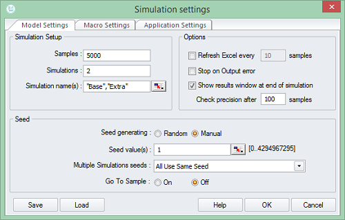
Simulation Setup group
Samples determines how many samples will be run for your model. 5000 samples is adequate to produce results of sufficient precision for most problems. If you need a specific level of precision in your results, use the Precision Control feature;
Simulations determines how many simulations will be run, each with the number of samples defined by the Samples dialog. It is more common to run just one simulation but, in conjunction with the VoseSimTable and/or the VoseCurrentSim functions, you can build models that will run several different scenarios together using this feature;Simulation names optionally allows you to give a name to each simulation for easier identification. Either enter a list of names, e.g.

or refer to a spreadsheet range which will copy the list in for you. If used, the name will appear in the Simulation # drop-down control in the Simulation Results window.
Options group
Refresh every … samples will update the Excel screen with the current simulated values every … samples. The option is switched off by default because it will slow down the simulation speed considerably, particularly if a small value (e.g. less than 1% of total samples to be run). If you wish to see numbers change on the screen (which can certainly capture people’s attention, particularly if one has imbedded graphs that change too), consider leaving this switched off for longer simulation runs and using the Update Screen control (the blue button at the bottom of the Simulation Progress control) which allows you to toggle switch screen updating on and off:
Stop on output error is a useful feature to debug your model. ModelRisk will stop simulating and show the scenario that produced the error.
Show results window at end of simulation will automatically pop up the Simulation Results window once ModelRisk has completed a simulation. This should normally be switched on, but you may want to deselect this option if, for example, you are only interested in the mean simulation result displayed by using VoseSimMean.
Seed group
Seed values are used to control how ModelRisk generates random samples for its stochastic variables. They are particularly useful if you wish to reproduce a set of simulation results.
Seed generating: Random will randomly select a different seed value. You can use this option, for example, to run multiple simulations of the same model with different seeds to see if there is any appreciable effect on the simulation results by using different random numbers;
Seed generating: Manual will use the seeds specified in the Seed Value(s) list
Seed Value(s) allows you to enter specific seed values. If you enter a list of values, the first value will be used in the first simulation run, etc. Seed values should be an integer between 0 and 4294967295 (2^32 -1)
Multiple simulation seeds has three options:
All use same seed: all simulations will use the first seed value specified in the Seed Value(s) field. If you use the same number of random variables in each simulation version of your model, this ensures that the difference is not due to random sampling
Use different seeds – First must be defined: the first simulation uses the first seed value specified in the Seed Value(s) field, and the remaining simulations will use different values. This helps evaluate whether the model results are materially affected by the random values being generated
Use different seeds – All must be defined: seed values for each simulation will use the list specified in the Seed Value(s) field. This can be useful if you wish to check the effect of using different seed values on your model, but is not commonly used.
Switching ON the Go To Sample feature will allow the user to load any simulation sample into the spreadsheet after the simulation has been performed. Switching this feature on might increase the simulation start time, and if this feature is not required, the user can switch it off to speed up the simulation.
If the feature if turned on, the Go To Sample functionality becomes available in the Data list view of the Results Viewer window.
Warning: The Go To Sample feature will not work properly if the spreadsheet model has any non-ModelRisk volatile functions (like Excel's RAND() function for example)
Save and Load group
You can save simulation settings, and load previously saved settings. The simulation settings file takes a .vmro extension.
Macro Settings Tab
The Macro settings tab controls VBA macros that are run before and after simulation samples and simulation runs. The tab allows specifying 4 places at which the VBA macros can be run:
1. Before each simulation
2. Before each sample
3. After each sample
4. After each simulation
The VBA macros can be chosen from the list of available macros saved in the current workbook:
Application Settings tab
Application settings control some basic ModelRisk default actions.
General group
Remove Vose Software details from reports will produce reports from the Results Viewer without any acknowledgment of the software used.
Save Results determines whether, when one saves a spreadsheet model for which a simulation has been performed, ModelRisk will prompt the user to save a simulation results file or do it automatically.
Simulation Settings group
Samples is the default number of samples that would be used for any newly created model.
The default number of samples is easily over-ridden by typing a different number in the ModelRisk ribbon, or in the Model Settings window.
Stop on output error determines the default setting, which can be over-ridden for an individual model run in the Model Settings window.
Show results window at end of simulation determines whether up the Simulation Results window will automatically pop once ModelRisk has completed a simulation. The setting can be over-ridden for an individual model run in the Model Settings window.
The Global timeout sets the maximum number of seconds for any ModelRisk function to calculate its value. It's useful when one uses calculation-intensive functions and enters parameters that result in a very long calculation loop.
Simulation Results group
Histogram Bars determines how many bars there will be in a histogram plot of simulation results. The Auto option will select the number of bars according to Sturges' rule to reflect the level of detail implied by the number of samples taken in a simulation run. The number of bars can still be changed for individual histogram plots in the Simulation Results window.
Histogram View determines whether the default plotting of histograms should be bars or lines. This can still be changed for individual histogram plots in the Simulation Results window. It is more common to use bars, but lines are better if you habitually plot several variables in the same histogram plot.
Histogram sliders determines the default location for sliders in terms of cumulative probabilities. This can still be changed for individual histogram plots in the Simulation Results window.
Box-plot percentiles determines the default percentiles plotted around the 50th percentile for box-plots. This can still be changed for individual histogram plots in the Simulation Results window.
Trend-plot percentiles determines the default percentiles plotted around the 50th percentile or mean for trend plots. This can still be changed for individual trend plots in the Simulation Results window.
Library group
Allow the user to set the location of the files created by the ModelRisk Library (Industrial edition only).
Navigation
- Risk management
- Risk management introduction
- What are risks and opportunities?
- Planning a risk analysis
- Clearly stating risk management questions
- Evaluating risk management options
- Introduction to risk analysis
- The quality of a risk analysis
- Using risk analysis to make better decisions
- Explaining a models assumptions
- Statistical descriptions of model outputs
- Simulation Statistical Results
- Preparing a risk analysis report
- Graphical descriptions of model outputs
- Presenting and using results introduction
- Statistical descriptions of model results
- Mean deviation (MD)
- Range
- Semi-variance and semi-standard deviation
- Kurtosis (K)
- Mean
- Skewness (S)
- Conditional mean
- Custom simulation statistics table
- Mode
- Cumulative percentiles
- Median
- Relative positioning of mode median and mean
- Variance
- Standard deviation
- Inter-percentile range
- Normalized measures of spread - the CofV
- Graphical descriptionss of model results
- Showing probability ranges
- Overlaying histogram plots
- Scatter plots
- Effect of varying number of bars
- Sturges rule
- Relationship between cdf and density (histogram) plots
- Difficulty of interpreting the vertical scale
- Stochastic dominance tests
- Risk-return plots
- Second order cumulative probability plot
- Ascending and descending cumulative plots
- Tornado plot
- Box Plot
- Cumulative distribution function (cdf)
- Probability density function (pdf)
- Crude sensitivity analysis for identifying important input distributions
- Pareto Plot
- Trend plot
- Probability mass function (pmf)
- Overlaying cdf plots
- Cumulative Plot
- Simulation data table
- Statistics table
- Histogram Plot
- Spider plot
- Determining the width of histogram bars
- Plotting a variable with discrete and continuous elements
- Smoothing a histogram plot
- Risk analysis modeling techniques
- Monte Carlo simulation
- Monte Carlo simulation introduction
- Monte Carlo simulation in ModelRisk
- Filtering simulation results
- Output/Input Window
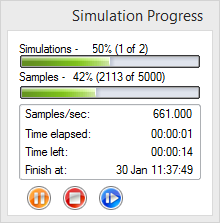
- Simulation Progress control
- Running multiple simulations
- Random number generation in ModelRisk
- Random sampling from input distributions
- How many Monte Carlo samples are enough?
- Probability distributions
- Distributions introduction
- Probability calculations in ModelRisk
- Selecting the appropriate distributions for your model
- List of distributions by category
- Distribution functions and the U parameter
- Univariate continuous distributions
- Beta distribution
- Beta Subjective distribution
- Four-parameter Beta distribution
- Bradford distribution
- Burr distribution
- Cauchy distribution
- Chi distribution
- Chi Squared distribution
- Continuous distributions introduction
- Continuous fitted distribution
- Cumulative ascending distribution
- Cumulative descending distribution
- Dagum distribution
- Erlang distribution
- Error distribution
- Error function distribution
- Exponential distribution
- Exponential family of distributions
- Extreme Value Minimum distribution
- Extreme Value Maximum distribution
- F distribution
- Fatigue Life distribution
- Gamma distribution
- Generalized Extreme Value distribution
- Generalized Logistic distribution
- Generalized Trapezoid Uniform (GTU) distribution
- Histogram distribution
- Hyperbolic-Secant distribution
- Inverse Gaussian distribution
- Johnson Bounded distribution
- Johnson Unbounded distribution
- Kernel Continuous Unbounded distribution
- Kumaraswamy distribution
- Kumaraswamy Four-parameter distribution
- Laplace distribution
- Levy distribution
- Lifetime Two-Parameter distribution
- Lifetime Three-Parameter distribution
- Lifetime Exponential distribution
- LogGamma distribution
- Logistic distribution
- LogLaplace distribution
- LogLogistic distribution
- LogLogistic Alternative parameter distribution
- LogNormal distribution
- LogNormal Alternative-parameter distribution
- LogNormal base B distribution
- LogNormal base E distribution
- LogTriangle distribution
- LogUniform distribution
- Noncentral Chi squared distribution
- Noncentral F distribution
- Normal distribution
- Normal distribution with alternative parameters
- Maxwell distribution
- Normal Mix distribution
- Relative distribution
- Ogive distribution
- Pareto (first kind) distribution
- Pareto (second kind) distribution
- Pearson Type 5 distribution
- Pearson Type 6 distribution
- Modified PERT distribution
- PERT distribution
- PERT Alternative-parameter distribution
- Reciprocal distribution
- Rayleigh distribution
- Skew Normal distribution
- Slash distribution
- SplitTriangle distribution
- Student-t distribution
- Three-parameter Student distribution
- Triangle distribution
- Triangle Alternative-parameter distribution
- Uniform distribution
- Weibull distribution
- Weibull Alternative-parameter distribution
- Three-Parameter Weibull distribution
- Univariate discrete distributions
- Discrete distributions introduction
- Bernoulli distribution
- Beta-Binomial distribution
- Beta-Geometric distribution
- Beta-Negative Binomial distribution
- Binomial distribution
- Burnt Finger Poisson distribution
- Delaporte distribution
- Discrete distribution
- Discrete Fitted distribution
- Discrete Uniform distribution
- Geometric distribution
- HypergeoM distribution
- Hypergeometric distribution
- HypergeoD distribution
- Inverse Hypergeometric distribution
- Logarithmic distribution
- Negative Binomial distribution
- Poisson distribution
- Poisson Uniform distribution
- Polya distribution
- Skellam distribution
- Step Uniform distribution
- Zero-modified counting distributions
- More on probability distributions
- Multivariate distributions
- Multivariate distributions introduction
- Dirichlet distribution
- Multinomial distribution
- Multivariate Hypergeometric distribution
- Multivariate Inverse Hypergeometric distribution type2
- Negative Multinomial distribution type 1
- Negative Multinomial distribution type 2
- Multivariate Inverse Hypergeometric distribution type1
- Multivariate Normal distribution
- More on probability distributions
- Approximating one distribution with another
- Approximations to the Inverse Hypergeometric Distribution
- Normal approximation to the Gamma Distribution
- Normal approximation to the Poisson Distribution
- Approximations to the Hypergeometric Distribution
- Stirlings formula for factorials
- Normal approximation to the Beta Distribution
- Approximation of one distribution with another
- Approximations to the Negative Binomial Distribution
- Normal approximation to the Student-t Distribution
- Approximations to the Binomial Distribution
- Normal_approximation_to_the_Binomial_distribution
- Poisson_approximation_to_the_Binomial_distribution
- Normal approximation to the Chi Squared Distribution
- Recursive formulas for discrete distributions
- Normal approximation to the Lognormal Distribution
- Normal approximations to other distributions
- Approximating one distribution with another
- Correlation modeling in risk analysis
- Common mistakes when adapting spreadsheet models for risk analysis
- More advanced risk analysis methods
- SIDs
- Modeling with objects
- ModelRisk database connectivity functions
- PK/PD modeling
- Value of information techniques
- Simulating with ordinary differential equations (ODEs)
- Optimization of stochastic models
- ModelRisk optimization extension introduction
- Optimization Settings
- Defining Simulation Requirements in an Optimization Model
- Defining Decision Constraints in an Optimization Model
- Optimization Progress control
- Defining Targets in an Optimization Model
- Defining Decision Variables in an Optimization Model
- Optimization Results
- Summing random variables
- Aggregate distributions introduction
- Aggregate modeling - Panjer's recursive method
- Adding correlation in aggregate calculations
- Sum of a random number of random variables
- Moments of an aggregate distribution
- Aggregate modeling in ModelRisk
- Aggregate modeling - Fast Fourier Transform (FFT) method
- How many random variables add up to a fixed total
- Aggregate modeling - compound Poisson approximation
- Aggregate modeling - De Pril's recursive method
- Testing and modeling causal relationships
- Stochastic time series
- Time series introduction
- Time series in ModelRisk
- Autoregressive models
- Thiel inequality coefficient
- Effect of an intervention at some uncertain point in time
- Log return of a Time Series
- Markov Chain models
- Seasonal time series
- Bounded random walk
- Time series modeling in finance
- Birth and death models
- Time series models with leading indicators
- Geometric Brownian Motion models
- Time series projection of events occurring randomly in time
- Simulation for six sigma
- ModelRisk's Six Sigma functions
- VoseSixSigmaCp
- VoseSixSigmaCpkLower
- VoseSixSigmaProbDefectShift
- VoseSixSigmaLowerBound
- VoseSixSigmaK
- VoseSixSigmaDefectShiftPPMUpper
- VoseSixSigmaDefectShiftPPMLower
- VoseSixSigmaDefectShiftPPM
- VoseSixSigmaCpm
- VoseSixSigmaSigmaLevel
- VoseSixSigmaCpkUpper
- VoseSixSigmaCpk
- VoseSixSigmaDefectPPM
- VoseSixSigmaProbDefectShiftLower
- VoseSixSigmaProbDefectShiftUpper
- VoseSixSigmaYield
- VoseSixSigmaUpperBound
- VoseSixSigmaZupper
- VoseSixSigmaZmin
- VoseSixSigmaZlower
- Modeling expert opinion
- Modeling expert opinion introduction
- Sources of error in subjective estimation
- Disaggregation
- Distributions used in modeling expert opinion
- A subjective estimate of a discrete quantity
- Incorporating differences in expert opinions
- Modeling opinion of a variable that covers several orders of magnitude
- Maximum entropy
- Probability theory and statistics
- Probability theory and statistics introduction
- Stochastic processes
- Stochastic processes introduction
- Poisson process
- Hypergeometric process
- The hypergeometric process
- Number in a sample with a particular characteristic in a hypergeometric process
- Number of hypergeometric samples to get a specific number of successes
- Number of samples taken to have an observed s in a hypergeometric process
- Estimate of population and sub-population sizes in a hypergeometric process
- The binomial process
- Renewal processes
- Mixture processes
- Martingales
- Estimating model parameters from data
- The basics
- Probability equations
- Probability theorems and useful concepts
- Probability parameters
- Probability rules and diagrams
- The definition of probability
- The basics of probability theory introduction
- Fitting probability models to data
- Fitting time series models to data
- Fitting correlation structures to data
- Fitting in ModelRisk
- Fitting probability distributions to data
- Fitting distributions to data
- Method of Moments (MoM)
- Check the quality of your data
- Kolmogorov-Smirnoff (K-S) Statistic
- Anderson-Darling (A-D) Statistic
- Goodness of fit statistics
- The Chi-Squared Goodness-of-Fit Statistic
- Determining the joint uncertainty distribution for parameters of a distribution
- Using Method of Moments with the Bootstrap
- Maximum Likelihood Estimates (MLEs)
- Fitting a distribution to truncated censored or binned data
- Critical Values and Confidence Intervals for Goodness-of-Fit Statistics
- Matching the properties of the variable and distribution
- Transforming discrete data before performing a parametric distribution fit
- Does a parametric distribution exist that is well known to fit this type of variable?
- Censored data
- Fitting a continuous non-parametric second-order distribution to data
- Goodness of Fit Plots
- Fitting a second order Normal distribution to data
- Using Goodness-of Fit Statistics to optimize Distribution Fitting
- Information criteria - SIC HQIC and AIC
- Fitting a second order parametric distribution to observed data
- Fitting a distribution for a continuous variable
- Does the random variable follow a stochastic process with a well-known model?
- Fitting a distribution for a discrete variable
- Fitting a discrete non-parametric second-order distribution to data
- Fitting a continuous non-parametric first-order distribution to data
- Fitting a first order parametric distribution to observed data
- Fitting a discrete non-parametric first-order distribution to data
- Fitting distributions to data
- Technical subjects
- Comparison of Classical and Bayesian methods
- Comparison of classic and Bayesian estimate of Normal distribution parameters
- Comparison of classic and Bayesian estimate of intensity lambda in a Poisson process
- Comparison of classic and Bayesian estimate of probability p in a binomial process
- Which technique should you use?
- Comparison of classic and Bayesian estimate of mean "time" beta in a Poisson process
- Classical statistics
- Bayesian
- Bootstrap
- The Bootstrap
- Linear regression parametric Bootstrap
- The Jackknife
- Multiple variables Bootstrap Example 2: Difference between two population means
- Linear regression non-parametric Bootstrap
- The parametric Bootstrap
- Bootstrap estimate of prevalence
- Estimating parameters for multiple variables
- Example: Parametric Bootstrap estimate of the mean of a Normal distribution with known standard deviation
- The non-parametric Bootstrap
- Example: Parametric Bootstrap estimate of mean number of calls per hour at a telephone exchange
- The Bootstrap likelihood function for Bayesian inference
- Multiple variables Bootstrap Example 1: Estimate of regression parameters
- Bayesian inference
- Uninformed priors
- Conjugate priors
- Prior distributions
- Bayesian analysis with threshold data
- Bayesian analysis example: gender of a random sample of people
- Informed prior
- Simulating a Bayesian inference calculation
- Hyperparameters
- Hyperparameter example: Micro-fractures on turbine blades
- Constructing a Bayesian inference posterior distribution in Excel
- Bayesian analysis example: Tigers in the jungle
- Markov chain Monte Carlo (MCMC) simulation
- Introduction to Bayesian inference concepts
- Bayesian estimate of the mean of a Normal distribution with known standard deviation
- Bayesian estimate of the mean of a Normal distribution with unknown standard deviation
- Determining prior distributions for correlated parameters
- Improper priors
- The Jacobian transformation
- Subjective prior based on data
- Taylor series approximation to a Bayesian posterior distribution
- Bayesian analysis example: The Monty Hall problem
- Determining prior distributions for uncorrelated parameters
- Subjective priors
- Normal approximation to the Beta posterior distribution
- Bayesian analysis example: identifying a weighted coin
- Bayesian estimate of the standard deviation of a Normal distribution with known mean
- Likelihood functions
- Bayesian estimate of the standard deviation of a Normal distribution with unknown mean
- Determining a prior distribution for a single parameter estimate
- Simulating from a constructed posterior distribution
- Bootstrap
- Comparison of Classical and Bayesian methods
- Analyzing and using data introduction
- Data Object
- Vose probability calculation
- Bayesian model averaging
- Miscellaneous
- Excel and ModelRisk model design and validation techniques
- Using range names for model clarity
- Color coding models for clarity
- Compare with known answers
- Checking units propagate correctly
- Stressing parameter values
- Model Validation and behavior introduction
- Informal auditing
- Analyzing outputs
- View random scenarios on screen and check for credibility
- Split up complex formulas (megaformulas)
- Building models that are efficient
- Comparing predictions against reality
- Numerical integration
- Comparing results of alternative models
- Building models that are easy to check and modify
- Model errors
- Model design introduction
- About array functions in Excel
- Excel and ModelRisk model design and validation techniques
- Monte Carlo simulation
- RISK ANALYSIS SOFTWARE
- Risk analysis software from Vose Software
- ModelRisk - risk modeling in Excel
- ModelRisk functions explained
- VoseCopulaOptimalFit and related functions
- VoseTimeOptimalFit and related functions
- VoseOptimalFit and related functions
- VoseXBounds
- VoseCLTSum
- VoseAggregateMoments
- VoseRawMoments
- VoseSkewness
- VoseMoments
- VoseKurtosis
- VoseAggregatePanjer
- VoseAggregateFFT
- VoseCombined
- VoseCopulaBiGumbel
- VoseCopulaBiClayton
- VoseCopulaBiNormal
- VoseCopulaBiT
- VoseKendallsTau
- VoseRiskEvent
- VoseCopulaBiFrank
- VoseCorrMatrix
- VoseRank
- VoseValidCorrmat
- VoseSpearman
- VoseCopulaData
- VoseCorrMatrixU
- VoseTimeSeasonalGBM
- VoseMarkovSample
- VoseMarkovMatrix
- VoseThielU
- VoseTimeEGARCH
- VoseTimeAPARCH
- VoseTimeARMA
- VoseTimeDeath
- VoseTimeAR1
- VoseTimeAR2
- VoseTimeARCH
- VoseTimeMA2
- VoseTimeGARCH
- VoseTimeGBMJDMR
- VoseTimePriceInflation
- VoseTimeGBMMR
- VoseTimeWageInflation
- VoseTimeLongTermInterestRate
- VoseTimeMA1
- VoseTimeGBM
- VoseTimeGBMJD
- VoseTimeShareYields
- VoseTimeYule
- VoseTimeShortTermInterestRate
- VoseDominance
- VoseLargest
- VoseSmallest
- VoseShift
- VoseStopSum
- VoseEigenValues
- VosePrincipleEsscher
- VoseAggregateMultiFFT
- VosePrincipleEV
- VoseCopulaMultiNormal
- VoseRunoff
- VosePrincipleRA
- VoseSumProduct
- VosePrincipleStdev
- VosePoissonLambda
- VoseBinomialP
- VosePBounds
- VoseAIC
- VoseHQIC
- VoseSIC
- VoseOgive1
- VoseFrequency
- VoseOgive2
- VoseNBootStdev
- VoseNBoot
- VoseSimulate
- VoseNBootPaired
- VoseAggregateMC
- VoseMean
- VoseStDev
- VoseAggregateMultiMoments
- VoseDeduct
- VoseExpression
- VoseLargestSet
- VoseKthSmallest
- VoseSmallestSet
- VoseKthLargest
- VoseNBootCofV
- VoseNBootPercentile
- VoseExtremeRange
- VoseNBootKurt
- VoseCopulaMultiClayton
- VoseNBootMean
- VoseTangentPortfolio
- VoseNBootVariance
- VoseNBootSkewness
- VoseIntegrate
- VoseInterpolate
- VoseCopulaMultiGumbel
- VoseCopulaMultiT
- VoseAggregateMultiMC
- VoseCopulaMultiFrank
- VoseTimeMultiMA1
- VoseTimeMultiMA2
- VoseTimeMultiGBM
- VoseTimeMultBEKK
- VoseAggregateDePril
- VoseTimeMultiAR1
- VoseTimeWilkie
- VoseTimeDividends
- VoseTimeMultiAR2
- VoseRuinFlag
- VoseRuinTime
- VoseDepletionShortfall
- VoseDepletion
- VoseDepletionFlag
- VoseDepletionTime
- VosejProduct
- VoseCholesky
- VoseTimeSimulate
- VoseNBootSeries
- VosejkProduct
- VoseRuinSeverity
- VoseRuin
- VosejkSum
- VoseTimeDividendsA
- VoseRuinNPV
- VoseTruncData
- VoseSample
- VoseIdentity
- VoseCopulaSimulate
- VoseSortA
- VoseFrequencyCumulA
- VoseAggregateDeduct
- VoseMeanExcessP
- VoseProb10
- VoseSpearmanU
- VoseSortD
- VoseFrequencyCumulD
- VoseRuinMaxSeverity
- VoseMeanExcessX
- VoseRawMoment3
- VosejSum
- VoseRawMoment4
- VoseNBootMoments
- VoseVariance
- VoseTimeShortTermInterestRateA
- VoseTimeLongTermInterestRateA
- VoseProb
- VoseDescription
- VoseCofV
- VoseAggregateProduct
- VoseEigenVectors
- VoseTimeWageInflationA
- VoseRawMoment1
- VosejSumInf
- VoseRawMoment2
- VoseShuffle
- VoseRollingStats
- VoseSplice
- VoseTSEmpiricalFit
- VoseTimeShareYieldsA
- VoseParameters
- VoseAggregateTranche
- VoseCovToCorr
- VoseCorrToCov
- VoseLLH
- VoseTimeSMEThreePoint
- VoseDataObject
- VoseCopulaDataSeries
- VoseDataRow
- VoseDataMin
- VoseDataMax
- VoseTimeSME2Perc
- VoseTimeSMEUniform
- VoseTimeSMESaturation
- VoseOutput
- VoseInput
- VoseTimeSMEPoisson
- VoseTimeBMAObject
- VoseBMAObject
- VoseBMAProb10
- VoseBMAProb
- VoseCopulaBMA
- VoseCopulaBMAObject
- VoseTimeEmpiricalFit
- VoseTimeBMA
- VoseBMA
- VoseSimKurtosis
- VoseOptConstraintMin
- VoseSimProbability
- VoseCurrentSample
- VoseCurrentSim
- VoseLibAssumption
- VoseLibReference
- VoseSimMoments
- VoseOptConstraintMax
- VoseSimMean
- VoseOptDecisionContinuous
- VoseOptRequirementEquals
- VoseOptRequirementMax
- VoseOptRequirementMin
- VoseOptTargetMinimize
- VoseOptConstraintEquals
- VoseSimVariance
- VoseSimSkewness
- VoseSimTable
- VoseSimCofV
- VoseSimPercentile
- VoseSimStDev
- VoseOptTargetValue
- VoseOptTargetMaximize
- VoseOptDecisionDiscrete
- VoseSimMSE
- VoseMin
- VoseMin
- VoseOptDecisionList
- VoseOptDecisionBoolean
- VoseOptRequirementBetween
- VoseOptConstraintBetween
- VoseSimMax
- VoseSimSemiVariance
- VoseSimSemiStdev
- VoseSimMeanDeviation
- VoseSimMin
- VoseSimCVARp
- VoseSimCVARx
- VoseSimCorrelation
- VoseSimCorrelationMatrix
- VoseOptConstraintString
- VoseOptCVARx
- VoseOptCVARp
- VoseOptPercentile
- VoseSimValue
- VoseSimStop
- Precision Control Functions
- VoseAggregateDiscrete
- VoseTimeMultiGARCH
- VoseTimeGBMVR
- VoseTimeGBMAJ
- VoseTimeGBMAJVR
- VoseSID
- Generalized Pareto Distribution (GPD)
- Generalized Pareto Distribution (GPD) Equations
- Three-Point Estimate Distribution
- Three-Point Estimate Distribution Equations
- VoseCalibrate
- ModelRisk interfaces
- Integrate
- Data Viewer
- Stochastic Dominance
- Library
- Correlation Matrix
- Portfolio Optimization Model
- Common elements of ModelRisk interfaces
- Risk Event
- Extreme Values
- Select Distribution
- Combined Distribution
- Aggregate Panjer
- Interpolate
- View Function
- Find Function
- Deduct
- Ogive
- AtRISK model converter
- Aggregate Multi FFT
- Stop Sum
- Crystal Ball model converter
- Aggregate Monte Carlo
- Splicing Distributions
- Subject Matter Expert (SME) Time Series Forecasts
- Aggregate Multivariate Monte Carlo
- Ordinary Differential Equation tool
- Aggregate FFT
- More on Conversion
- Multivariate Copula
- Bivariate Copula
- Univariate Time Series
- Modeling expert opinion in ModelRisk
- Multivariate Time Series
- Sum Product
- Aggregate DePril
- Aggregate Discrete
- Expert
- ModelRisk introduction
- Building and running a simple example model
- Distributions in ModelRisk
- List of all ModelRisk functions
- Custom applications and macros
- ModelRisk functions explained
- Tamara - project risk analysis
- Introduction to Tamara project risk analysis software
- Launching Tamara
- Importing a schedule
- Assigning uncertainty to the amount of work in the project
- Assigning uncertainty to productivity levels in the project
- Adding risk events to the project schedule
- Adding cost uncertainty to the project schedule
- Saving the Tamara model
- Running a Monte Carlo simulation in Tamara
- Reviewing the simulation results in Tamara
- Using Tamara results for cost and financial risk analysis
- Creating, updating and distributing a Tamara report
- Tips for creating a schedule model suitable for Monte Carlo simulation
- Random number generator and sampling algorithms used in Tamara
- Probability distributions used in Tamara
- Correlation with project schedule risk analysis
- Pelican - enterprise risk management