Tips for creating a schedule model suitable for Monte Carlo simulation

The first step in performing a risk analysis of your project schedule is to create a basic schedule model in either Oracle Primavera or Microsoft Project. There are several things to consider in building such a model:

• Use an appropriate schedule logic with start and end milestones

• Include tasks that may or may not occur

• Assign most likely estimates of task durations

• Assign tasks to work breakdown structures (WBSs) if possible

• Create parent and child task structures at various levels for large schedules

• Add milestones anywhere you would like to get estimates of finish dates

• Ensure the schedule is sufficiently detailed to be able to pinpoint exactly where a risk event may affect the schedule

Schedule logic

Monte Carlo simulation on project schedules is most easily performed when one only uses Finish-Start relationships, which have a causal and temporal logic that is easy to understand. However, project schedules can be built with a number of dependency relationships for defining when a task starts and finishes. Tamara can interpret any network logic you use, but because Tamara runs Monte Carlo simulations – randomly changing the durations of tasks and adding/removing risk events – logic other than Finish-Start can produce unexpected logical conflicts not present in the baseline model created in Primavera or MS Project.

Relationships linking tasks

A good quality schedule model will have the various tasks linked together with some logic. In particular, there should be no tasks for which the finish date is not somehow linked to the estimated end of the project. The types of linkage are:

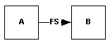
FS: Finish(A)-Start(B)

This is the most common dependency logic, the method recommended in project planning best practice, and the one we strongly encourage you to use. It says that Task A must be complete before Task B can start. All projects can be structured into a Finish-Start network with a bit of care.

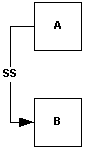
SS: Start(A)-Start(B)

This means that neither task can start without the other. In general, it really means that both tasks are waiting for some other trigger (like getting approval to proceed). It is better to model the relationship explicitly with the trigger event using Finish-Start logic, even if this trigger event has a duration of zero.

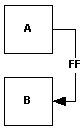
FF: Finish(A)-Finish(B)

This mean that neither can finish without the other. It is an approximation to the situation where both tasks need to be integrated together (another task that depends on both A and B being complete).

Lags

This means that one is waiting for something to happen, e.g. approval after submission, which is not being explicitly incorporated into the schedule model. We recommend that lags are avoided in schedule models built for Tamara, and the event that is being waited for is explicitly included.

Negative lags

Finish-Start logic is sometimes defined with a negative lag, meaning that task B will start when Task A finishes, minus some time (i.e. sometime before Task A is finished). Negative lags should be very much avoided. In reality, we cannot know when Task A will finish with certainty until it has actually done so.  This becomes important when uncertainty is incorporated into the schedule as it can create some logical inconsistencies – e.g. when the negative lag is shorter than the simulated duration of Task A.

The usual reason for including negative lags is that one wants to plan a task to start in parallel with its predecessor after a certain amount of progress has been achieved on the predecessor. It is better to split Task A into two, and model Task B as starting when the first part of Task A is complete. 

Positive lags

Finish-Start logic is sometimes defined with a positive lag, meaning that task B will start when Task A finishes plus some time. The usual reason for including positive lags in Finish-Start logic is that the lag is effectively representing another task, or set of tasks, that are not explicitly being modelled. We recommend that one explicitly models these extra tasks if possible.

Fixed start or finish dates

Fixed-value schedule models (i.e. models with no uncertainty) often include ‘hard’ start or finish dates. This implies that there is no uncertainty about these dates. Reality is often different, so you should be very careful about including these ‘hard’ values.

Tamara will respect any fixed dates that you include in the model, so be aware that this could lead to an unrealistic result, particularly if you see that Tamara is simulating a task to be finished very often on the hard finish date (and starting on the hard finish date). This implies that Tamara is being forced to finish a task on a specific date, even if reality says that there is a high probability it would exceed that date.

Grouping tasks

A key failure of schedule risk analysis modelling in the past has been to acknowledge systemic uncertainty drivers that can affect large parts of your project at the same time. For example, you may be using a contractor to install all the IT for your project. There may be many different tasks for which some IT involvement is necessary. If the contractor turned out to be very slow, disorganized, or unskilled, many activities in your project could be adversely affected.

Tamara provides a unique way to deal with this that is easy to implement, simple to understand, and quick to execute even for extremely large schedules. In order to take advantage of this capability, group tasks into categories in the baseline schedule model built with primavera or MS Project. You can use WBS, CBS and other labels for this. Examples would be: ‘welding’, ‘detailed engineering’, ‘procurement of raw materials’, etc.

Incorporating potential activities

Some activities may or may not need to be undertaken, for example redesigning some part of the system after initial testing. These activities should be included within the baseline model. If they are unlikely to occur, set the duration to zero in the baseline model. Tamara will allow you to assign a probability of their occurrence and an uncertain duration later.

Save the baseline schedule model

Remember to save the model in a location that the Tamara user will have access to. Tamara can access project plan models from Primavera and Project servers, as well as single model files stored on a drive.