The quality of a risk analysis

See also: Risk management introduction

Risk analyses are often of poor quality. They might also be very expensive, take a long time to complete and use up valuable human resources. In fact, the more complex and expensive a quantitative risk analysis is, the more likely it is to be of poor quality. Worst of all, the people making decisions on the results of these analyses have little if any idea of how bad they are. These are rather attention-grabbing sentences but this topic is small and you really should not to skip over it: it could save you a lot of heartache.

The reasons a risk analysis can be terrible

To give some motivation for this topic, let us look at some of the results of a survey we ran some years ago in a well-developed science-based area of risk analysis. The question appears in the title of each pane. Which results do you find most worrying?

 

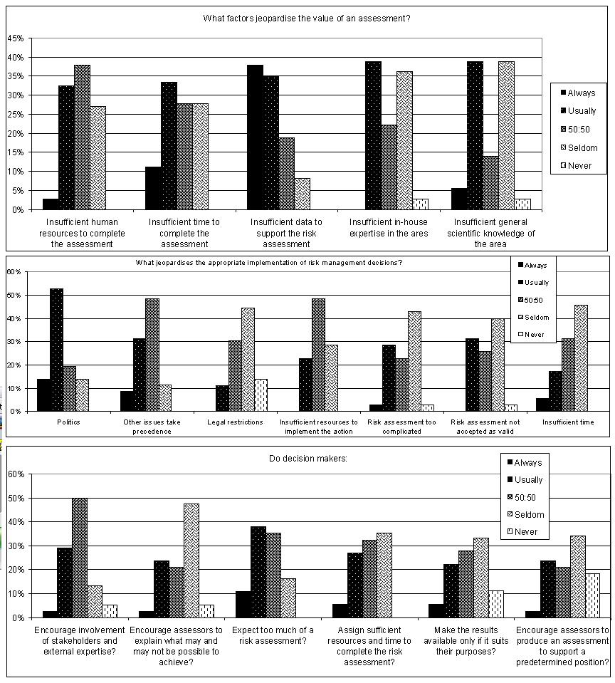
From the first of the figures above you'll see that there really needs to be more communication between decision-makers and their risk analysts and a greater attempt to work as a team. The risk analyst can be an important liaison between those 'on the ground' who understand the problem at hand and hold the data and those who make decisions. The risk analyst needs to understand the context of the decision question and have the flexibility to be able to find the method of analysis that gives the most useful information. Too often risk analysts complain that they get told to produce a quantitative model by the boss, but have to make the numbers up because the data aren't there. Now doesn't that seem silly? Surely the decision-maker would be none too happy to know the numbers are all made up, but the risk analyst is often not given access to the decision-makers to let them know. On the other hand, in some business and regulatory environments they are trying to follow a rule that says a quantitative risk analysis needs to be completed - the box needs ticking.

Regulations and guidelines can be a real impediment to creative thinking. Our founder, David Vose, has been in plenty of committees gathered to write risk analysis guidelines and he does his best to reverse the tendency to be formulaic. His argument is that in well over twenty years he have never done the same risk analysis twice: every one has its individual peculiarities. Risk analysis should not be a packaged commodity but a voyage of reasoned thinking leading to the best possible decision at the time.

It is usually pretty easy to see early on in the risk analysis process that a quantitative risk analysis will be of little value. There are several key areas where it can fall down:

1. It can't answer all the key questions;

2. There are going to be a lot of assumptions;

3. There is going to be one or more show-stopping assumption; and

4. There aren't enough good data or experts.

One can get around (1) sometimes by doing different risk analyses for different questions, but that can be problematic when each risk analysis has a different set of fundamental assumptions - how do we compare their results?

For (2) you need to have some way of expressing whether a lot of little assumptions compound to make a very vulnerable analysis: if you have 20 assumptions (and 20 is quite a small number), all pretty good ones - e.g. we think there's a 90% chance they are correct, but the analysis is only useful if all the assumptions are correct, then we only have a 0.9²⁰ = 12% chance that the assumption set is correct. Of course, if this was the real problem we wouldn't bother writing models. In reality, in the business world particularly, we deal with assumptions that are good enough because the answers we get are close enough. In some more scientific areas, like human health, we have to deal with assumptions like: compound X is present; compound X is toxic; people are exposed to compound X; the exposure is sufficient to cause harm; and treatment is ineffective. The sequence then produces the theoretical human harm we might want to protect against, but if any one of those assumptions is wrong there is no human health threat to worry about.

If (3) occurs we have a pretty good indication that we don't know enough to produce a decent risk analysis model, but maybe we can produce two or three crude models under different possible assumptions and see whether we come to the same conclusion anyway.

(4) is the least predictable area because the risk analyst doing a preliminary scoping can be reassured that the relevant data are available, but then finds out they are not available either because the data turn out to be clearly wrong (one sees this a lot, even in peer-reviewed work), the data aren't what was thought, there is a delay past the deadline in the data becoming available, or the data are dirty and need so much rework that it becomes impractical to analyze them within the decision timeframe.

There is a lot of emphasis placed on transparency in a risk analysis, which usually manifests itself in a large report describing the model, all the data and sources, the assumptions, etc. and then finishes with some graphical and numerical risk analysis outputs. I've seen reports of one or two hundred pages and that seem far from transparent to me - who really has the time or inclination to read such a document? The executive summary tends to focus on the decision question and numerical results, and places little emphasis on the robustness of the study.

Communicating quality of data

Elsewhere in this help file you will find lots of techniques for describing the numerical accuracy that a model can provide given the data that are available. These analyses are at the heart of a quantitative risk analysis and give us distributions, percentiles, sensitivity plots, etc.

We will now look at how to communicate any impact on the robustness of a model due to the assumptions behind using data or settling on a model scope and structure. We encourage the risk analyst to write down each assumption that is made in developing equations and performing statistical analyses.

We get participants to do the same in the training courses we teach as they solve simple class exercises and there is a general surprise at how many assumptions are implicit in even the simplest type of equations. It becomes rather onerous to write all these assumptions down, but it is even more difficult to convert the conceptual assumptions underpinning our probability models into something that a reader rather less familiar with probability modelling might understand.

The NUSAP method (Numeral Unit Spread Assessment Pedigree, Funtowicz and Ravetz, 1990) is a notational system that communicates the level of uncertainty for data in scientific analysis used for policy making.  The idea is to use a number of experts in the field to score independently the data under different categories. The system is well-established as being useful in toxicological risk assessment. We describe here a generalization of the idea. It's key attractions are that it is easy to implement and can be summarised into consistent pictorial representations.

In the table below we used the categorisation descriptions of data from van der Sluijs et al (2005), which are: proxy - reflecting how close data being used are to ideal; empirical - reflecting the quantity and quality of the data; method - reflecting where the method used to collect the data lay between careful and well-established, and haphazard; and validation - reflecting whether the acquired data have been matched to real world experience (e.g. does an effect observed in a laboratory actually occur in the wider world).

Pedigree matrix for parameter strength (adapted from Boone et al, 2007).

Each data set is scored in turn by each expert. The average of all scores is calculated and then divided by the maximum attainable score of 4. For example:

	Proxy	Empirical	Method	Validation
Expert A	3	2	4	3
Expert B	3	2	4	3
Expert C	2	1	3	4

gives an average score of 2.833. Dividing by the maximum score of 4 gives 0.708. An additional level of sophistication is to allow the experts to weight their level of expertise for the particular variable in question (e.g. 0.3 for low, 0.6 for medium and 1.0 for high, as well as allowing experts to select not to make any comment when it is outside their competence) in which case one calculates a weighted average score. One can then plot these scores together and segregate them by different parts of the analysis if desired, which gives an overview of the robustness of data used in the analysis:

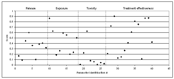
Plot of average scores for data sets in a toxicological risk assessment

Scores can be generally categorized as follows:

<0.2                weak

0.2 - 0.4          moderate

>0.4 - 0.8        high

>0.8                excellent

We can summarize the scores for each data set using a kite diagram to give a visual 'traffic light' green representing the parameter support is excellent, red representing weak, and one or two levels of orange representing gradations between these extremes. The figure below gives an example: one works from the centre point marking on the axes the weighted fraction of all the experts considering the parameter support to be 'excellent', then add the weighted fraction considering the support to be 'high' etc. These points are then joined to make the different color zones - from green in the centre for 'excellent', through yellow and orange, to red in the last category: a kite will be green if all experts agree the parameter support is excellent and red for weak.

Plotting these kite diagrams together can give a strong visual representation: a sea of green should give great confidence, a sea of red says the risk analysis is extremely weak. In practice, we'll end up with a big mix of colors but over time one can get a sense of what color mix is typical, when an analysis is comparatively weak or strong, and when it can be relied upon for your field.

 

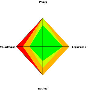
Summarizing the level of data support the experts believe that a model parameter will have: red (dark) in the outer ban = weak; green (light) in the inner band = excellent.

The only real impediment to using the system above is that you need to develop a database software tool. We have developed the Pelican risk management system for this purpose.

Level of criticality

The categorisation system described above helps determine whether a parameter is well-supported, but it can still misrepresent the robustness of the risk analysis. For example, we might have done a food safety microbial risk analysis involving ten parameters - nine enjoy high or excellent support, and one is suffering weak support. If that weakly supported parameter is defining the dose-response relationship (the probability a random individual will experience an adverse health effect given the number of pathogenic organisms ingested) then the whole risk analysis is jeopardized because the dose-response is the link between all the exposure pathways and the amount of pathogen involved (often a big model), and the size of human health impact that results. It is therefore rather useful to separate the kite diagrams and other analyses into different categories for the level of dependence the analysis has on each parameter: critical, important and small, for example.

A more sophisticated version for separating the level of dependence is to statistically analyze the degree of effect each parameter has on the numerical result: for example, one might look at the difference in the mean of the model output when the parameter distribution is replaced by its 95^th and 5^th percentile. Take that range and multiply by (1-the support score, giving 0 for excellent, 1 for terrible), gives one a sense of the level of vulnerability of the output numbers. However, this method suffers other problems. Imagine that we are performing a risk analysis on an emerging bacterium for which we have absolutely no dose-response data so we use a data set for a surrogate bacterium that we think will have a very similar effect (e.g. because it produces a similar toxin). We might have large amounts of excellent data for the surrogate bacterium and may therefore have little uncertainty about the dose-response model so using the 5^th and 95^th percentiles of the uncertainty about that dose-response model will result in a small change in the output and multiplying that by (1-the support score) will under-represent the real uncertainty. A second problem is that we often estimate two or more model parameters from the same data set: for example, a dose-response model often has two or three parameters that are fitted to data. Each parameter might be quite uncertain but the dose-response curve can be nonetheless quite stable, so this numerical analysis needs to look at the combined effect of the uncertain parameters as a single entity which requires a fair bit of number juggling.

The biggest uncertainty in a risk analysis

The techniques discussed above have focused on the vulnerability of the results of a risk analysis to the parameters of a model. When we are asked to review or audit a risk analysis the client is often surprised that our first step is not to look at the model mathematics and supporting statistical analyses, but to consider what the decision questions are, whether there were a number of assumptions, whether it would be possible to do the analysis a different (usually simpler, but sometimes more complex and precise) way, whether this other way would give the same answers and see if there are any means for comparing predictions against reality. What we are trying to do is see whether the structure and scope of the analysis is correct. The biggest uncertainty in a risk analysis is whether we started off analyzing the right thing and in the right way.

Finding the answer is very often not amenable to any numerical technique because we will not have any alternative to compare against. If we do, it might nonetheless take a great deal of effort to put together an alternative risk analysis model and a model audit is usually too late in the process to be able to start again. A much better idea, in my view, is to get a sense at the beginning of a risk analysis, on how confident we should be that the analysis will be scoped sufficiently broadly, or how confident we are that the world is adequately represented by our model. Needless to say, we can also start rather confident that our approach will be quite adequate and then, once having delved in to the details of the problem, find out we were quite mistaken so it is important to keep revisiting our view of the appropriateness of the model.

We encourage clients, particularly in the scientific areas of risk that we work in, to instigate a solid brainstorming session of experts and decision-makers whenever it has been decided that a risk analysis is to be undertaken, or maybe is just under consideration.

The focus is to discuss the form and scope of the potential risk analysis.

The experts first of all need to think about the decision-questions, discuss with decision-makers any possible alternatives or supplements to those questions and then consider how they can be answered, and what the outputs should look like (e.g. only the mean is required, or some high percentile). Each approach will have a set of assumptions which need to be thought through carefully: what would the effect be if the assumptions are wrong? If we use a conservative assumption and estimate a risk that is too high, are we back to where we started? We need to think about data requirements too: are the quality likely to be good and the data easily attainable?

When the brainstorming is over, we recommend that you pass around a questionnaire to each expert and ask those attending to independently answer a questionnaire something like this:

We discussed three risk analysis approaches (description A, description B, description C). Please indicate your level of confidence (0 = none, 1 = slight, 2 = good, 3 = excellent, -1 = no opinion) to the following:

1. What is your confidence that Method (A,...B,C) will be sufficiently flexible and comprehensive to answer any foreseeable questions from the management about this risk?

2. What is your confidence that Method (A,...B,C) is based on assumptions that are correct?

3. What is your confidence for Method (A,...B,C) that the necessary data will be available within the required timeframe and budget?

4. What is your confidence that the Method (A,...B,C) analysis will be completed in time?

5. What is your confidence that there will be strong support for Method (A,...B,C) among reviewing peers?

6. What is your confidence that there will be strong support for Method (A,...B,C) among stakeholders?

Asking each brainstorming participant independently will help you attain a balanced view, particularly if the chairperson of that meeting has enforced the discipline of requiring participants not to express their view on the above questions during the meeting (it won't be completely possible, but you are trying to make sure that nobody will be influenced into giving a desired answer). Asking people independently rather than trying to achieve consensus during the meeting will also help remove the over-confidence that often appears when people make a group decision.

Iterate

Things change. The political landscape in which the decision is to be made can become more hostile or accepting to some assumptions, data can prove better or worse than we initially thought, new data turn up, new questions suddenly become important, the time frame or budget can change, etc.

So it makes sense to go back from time to time over the types of assumptions analysis discussed above and to remain open to taking a different approach, even to making as dramatic a change as going from a quantitative to a qualitative risk analysis. That means you (analysts and decision makers alike) should also be a little guarded in making premature promises so you have some space to adapt. In our consultancy contracts, for example, a client will usually commission us to do a quantitative risk analysis and tell us about the data they have. We'll probably have had a little look at the data too. We prefer to structure our proposal into stages.

In the first stage we go over the decision problem, review any constraints and (time, money, political, etc.), take a first decent look at the available data, and figure out possible ways of getting to the answer. Then we produce a report describing how we want to tackle the problem and why. At that stage the client can stop the work, continue with us, do it themselves, or maybe hire someone else if they wish. It may take a little longer (usually a day or two) but everyone's expectations are kept realistic, we are not cornered into doing a risk analysis that we know is inappropriate, and clients don't waste their time or money. As consultants we are in the somewhat privileged position of turning down work that we know would be terrible. A risk analyst employed by a company or government department may not have that luxury.

 

---

© Vose Software™ 2017. Reference Number: M-M0919-A