Your First Model
ModelRisk is a risk analysis and Moonte Carlo simulation add-in for Excel. This topic is aimed at the risk analysis novice and introduces the very basics of building a Monte Carlo simulation model to get you started.
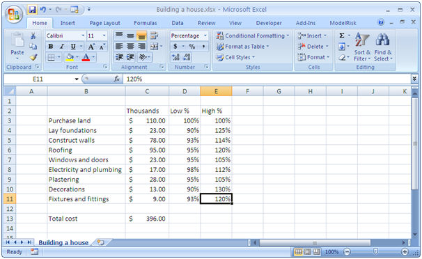
We begin with the following spreadsheet model for the cost of building
a house. The finished model can be downloaded ![]() here. Column C contains your best guess
at how much each element of the project might cost, summing to a total
of $396,000 in Cell C13.
here. Column C contains your best guess
at how much each element of the project might cost, summing to a total
of $396,000 in Cell C13.
However, these are just best guesses and the actual cost could be higher or low. For example, you might already have agreed purchase of the land, so the price is known, but the cost of laying the foundations might be up to 10% lower, or 25% higher. We can build a couple of extra columns showing the percentage range:
Add distributions
In another column we now add ModelRisk functions that will generate random values around those ranges with a most likely value of 100% by clicking the Select Distribution button:

This opens up a dialog in which we can chose from a very wide range of distributions. In this case, the Subjective group of distributions is most appropriate because these are subjective estimates:
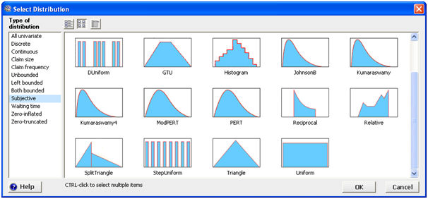
The most common choices would be a PERT or Triangle distribution because they are defined by their minimum, mode (most likely) and maximum values – the information that we have in this model. We’ll pick both by using CTRL-click and then OK.
ModelRisk plots these two distributions together. We can link each distribution’s parameter values to cells in Excel:

Let’s say that the Triangle distribution better reflects your opinion
because it gives more probability to the right hand side of the range.
Select the Triangle (by clicking on its name, highlighted here in pink)
and then click on  to insert
the Triangle distribution into the correct model cell. There are several
options available at this point:
to insert
the Triangle distribution into the correct model cell. There are several
options available at this point:

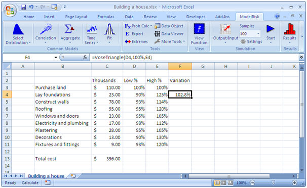
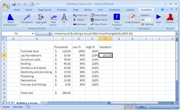
‘Distribution’ is the most commonly used, which will insert a function in Excel that will randomly generate values from this distribution. Cell F4 (the selected location) now displays a VoseTriangle distribution with minimum, mode and maximum values of 90% (D4), 100%, and 125% (E4) respectively.
Define inputs
We will name this cell as an input distribution to the model by clicking on the Output/Input button:

The following dialog box appears:
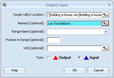
Here we select Cell B4 for the Name field, select Input rather than Output, and click OK. The cell formula has now changed to include a VoseInput function. This function does not alter the calculation in any ways, but is useful in a later stage discussed below.
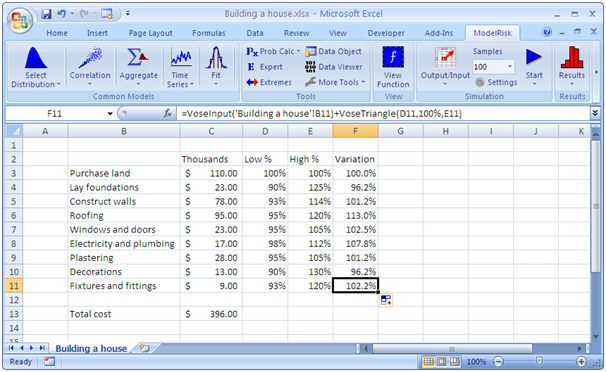
We can now copy this formula through the rest of the column:
Next, we write a new formula to calculate the total project cost with these random variations from the most likely values. In this case, we will use Excel’s SUMPRODUCT function:

Define outputs
Finally, since this is the focus of our problem, we name the cell as a ModelRisk output – using the same Outputs/Inputs dialog as before but now selecting the Output rather than Input option. The final formula in cell F13 now becomes:
=VoseOutput(D13)+SUMPRODUCT(C3:C11,F3:F11)
The model is finished. Now it is time to analyze what it can tell us.
Run the model
In order to understand how much uncertainty there is in the total cost of the project we need to run a Monte Carlo simulation – which results in a large set of probabilistically weighted ‘what-if’ scenarios by picking different random values from each of the model’s distributions and calculating the total cost each time.
To run a simulation in ModelRisk, simply select the number of samples to run in the ribbon dialog (in the screenshot above it is set to 100, which we’ll change to 50,000) and then click on:

ModelRisk will then run 50,000 Monte Carlo ‘samples’, which takes about 14 seconds.
View the results
When the simulation has finished, ModelRisk will open the Results Viewer window:
On the left is a list of the named outputs and inputs of the model (i.e. those cells containing a VoseOutput or VoseInput function). On the right is a graph of the output (total cost) and at the bottom a list of pages. One can add more pages by clicking the right-most tab.
The original $396,000 estimate based on adding the best guess values
is quite far to the left, meaning that there is a high probability of
the project costing more. We can see what that probability is, by moving
the sliders, and also find a more realistic budget by clicking the  icon above the graph which opens the following dialog:
Here, we have entered the original $396,000 value and asked for a budget for which there is a 90% probability the actual cost will fall below. Click OK, and the sliders move to reflect these changes:

It shows that, given the assumptions made earlier, there is only about a 6% chance of falling below the original estimate, and that there is only 10% probability of exceeding a more conservative budget of $415,000.
Sensitivity analysis
The histogram plot shows that the total cost might lie anywhere between around $390,000 and $425,000. You might well be interested in knowing which of the costs is driving this uncertainty, which is the purpose of performing a sensitivity analysis. ModelRisk offers many variations on sensitivity analysis because it is a very important component of risk-based decision making. We’ll look at just two here.
The first type of sensitivity analysis is a tornado chart, which ModelRisk will generate by clicking this icon:

resulting in the following plot:
This plot shows the sensitivity of the 90th percentile of the total cost distribution to each input distribution. It shows that roofing costs drive the project cost uncertainty the most. If the roofing cost is low, the project cost’s 90th percentile is around $404,000, and if the roofing cost is high, the project cost’s 90th percentile is around $422,000 – a wider range than for any other input variable.
The second type of sensitivity analysis is called a Spider Plot, which ModelRisk will generate by clicking this icon:

resulting in the following plot:
This plot gives more detailed information than the Tornado Plot. Here we are looking at the sensitivity to each input of the mean total cost (the mean is the ‘balance point’ of the histogram distribution, we could also look at a percentile or other statistical attributes). Again, it shows that roofing costs are dominant because it gives the greatest vertical range. In this problem, we are dealing with costs so there is a linear relationship between the inputs and the output, reflected in lines that increase from bottom left to top right in the plot, but in more involved problems a spider plot can reveal more complex relationships.
From analysis to decision
The analysis clearly provides some important information for a decision maker:
1. The budget should be set closer to $420,000 to be reasonably sure of having the cash available to complete the project
2. It is probably worth investigating whether it is possible to reduce the uncertainty on roofing costs (as well as the wall construction and laying the foundation) because these will firm up the cost estimate considerably.
Next steps in learning to use ModelRisk and risk analysis
ModelRisk has a very extensive range of risk analysis tools for you to explore. For example, in the model described in this document, perhaps the major driver behind the roofing and wall construction uncertainty is the competence of the contractor – and the same contractor is doing both parts of the project. That means that if the contractor turns out to be incompetent it will affect both parts of the project adversely – in other words, there is a correlation between these two input variables that needs to be described because it will increase the uncertainty of the total cost estimate. ModelRisk offers a range of correlation tools to build correlation relationships.
You might have a lot of data you wish to use to support your risk analysis. ModelRisk offers advanced yet user-friendly tools for fitting distributions, correlations, and time series – as well as a range of features to statistically and visually explore your data.
ModelRisk also comes with a very extensive help file that you can browse and search through. There are a wide variety of example models you can work through too. Vose Software (www.vosesoftware.com) and our reseller network also provide in-house and public training courses in building risk analysis models – and using them to make decisions. The courses are written and presented by professional risk analysts, so while you learn to use ModelRisk you will also benefit from the real world experience of a seasoned risk analyst.
You can also download this topic in PDF format.
Navigation
- Risk management
- Risk management introduction
- What are risks and opportunities?
- Planning a risk analysis
- Clearly stating risk management questions
- Evaluating risk management options
- Introduction to risk analysis
- The quality of a risk analysis
- Using risk analysis to make better decisions
- Explaining a models assumptions
- Statistical descriptions of model outputs
- Simulation Statistical Results
- Preparing a risk analysis report
- Graphical descriptions of model outputs
- Presenting and using results introduction
- Statistical descriptions of model results
- Mean deviation (MD)
- Range
- Semi-variance and semi-standard deviation
- Kurtosis (K)
- Mean
- Skewness (S)
- Conditional mean
- Custom simulation statistics table
- Mode
- Cumulative percentiles
- Median
- Relative positioning of mode median and mean
- Variance
- Standard deviation
- Inter-percentile range
- Normalized measures of spread - the CofV
- Graphical descriptionss of model results
- Showing probability ranges
- Overlaying histogram plots
- Scatter plots
- Effect of varying number of bars
- Sturges rule
- Relationship between cdf and density (histogram) plots
- Difficulty of interpreting the vertical scale
- Stochastic dominance tests
- Risk-return plots
- Second order cumulative probability plot
- Ascending and descending cumulative plots
- Tornado plot
- Box Plot
- Cumulative distribution function (cdf)
- Probability density function (pdf)
- Crude sensitivity analysis for identifying important input distributions
- Pareto Plot
- Trend plot
- Probability mass function (pmf)
- Overlaying cdf plots
- Cumulative Plot
- Simulation data table
- Statistics table
- Histogram Plot
- Spider plot
- Determining the width of histogram bars
- Plotting a variable with discrete and continuous elements
- Smoothing a histogram plot
- Risk analysis modeling techniques
- Monte Carlo simulation
- Monte Carlo simulation introduction
- Monte Carlo simulation in ModelRisk
- Filtering simulation results
- Output/Input Window
- Simulation Progress control
- Running multiple simulations
- Random number generation in ModelRisk
- Random sampling from input distributions
- How many Monte Carlo samples are enough?
- Probability distributions
- Distributions introduction
- Probability calculations in ModelRisk
- Selecting the appropriate distributions for your model
- List of distributions by category
- Distribution functions and the U parameter
- Univariate continuous distributions
- Beta distribution
- Beta Subjective distribution
- Four-parameter Beta distribution
- Bradford distribution
- Burr distribution
- Cauchy distribution
- Chi distribution
- Chi Squared distribution
- Continuous distributions introduction
- Continuous fitted distribution
- Cumulative ascending distribution
- Cumulative descending distribution
- Dagum distribution
- Erlang distribution
- Error distribution
- Error function distribution
- Exponential distribution
- Exponential family of distributions
- Extreme Value Minimum distribution
- Extreme Value Maximum distribution
- F distribution
- Fatigue Life distribution
- Gamma distribution
- Generalized Extreme Value distribution
- Generalized Logistic distribution
- Generalized Trapezoid Uniform (GTU) distribution
- Histogram distribution
- Hyperbolic-Secant distribution
- Inverse Gaussian distribution
- Johnson Bounded distribution
- Johnson Unbounded distribution
- Kernel Continuous Unbounded distribution
- Kumaraswamy distribution
- Kumaraswamy Four-parameter distribution
- Laplace distribution
- Levy distribution
- Lifetime Two-Parameter distribution
- Lifetime Three-Parameter distribution
- Lifetime Exponential distribution
- LogGamma distribution
- Logistic distribution
- LogLaplace distribution
- LogLogistic distribution
- LogLogistic Alternative parameter distribution
- LogNormal distribution
- LogNormal Alternative-parameter distribution
- LogNormal base B distribution
- LogNormal base E distribution
- LogTriangle distribution
- LogUniform distribution
- Noncentral Chi squared distribution
- Noncentral F distribution
- Normal distribution
- Normal distribution with alternative parameters
- Maxwell distribution
- Normal Mix distribution
- Relative distribution
- Ogive distribution
- Pareto (first kind) distribution
- Pareto (second kind) distribution
- Pearson Type 5 distribution
- Pearson Type 6 distribution
- Modified PERT distribution
- PERT distribution
- PERT Alternative-parameter distribution
- Reciprocal distribution
- Rayleigh distribution
- Skew Normal distribution
- Slash distribution
- SplitTriangle distribution
- Student-t distribution
- Three-parameter Student distribution
- Triangle distribution
- Triangle Alternative-parameter distribution
- Uniform distribution
- Weibull distribution
- Weibull Alternative-parameter distribution
- Three-Parameter Weibull distribution
- Univariate discrete distributions
- Discrete distributions introduction
- Bernoulli distribution
- Beta-Binomial distribution
- Beta-Geometric distribution
- Beta-Negative Binomial distribution
- Binomial distribution
- Burnt Finger Poisson distribution
- Delaporte distribution
- Discrete distribution
- Discrete Fitted distribution
- Discrete Uniform distribution
- Geometric distribution
- HypergeoM distribution
- Hypergeometric distribution
- HypergeoD distribution
- Inverse Hypergeometric distribution
- Logarithmic distribution
- Negative Binomial distribution
- Poisson distribution
- Poisson Uniform distribution
- Polya distribution
- Skellam distribution
- Step Uniform distribution
- Zero-modified counting distributions
- More on probability distributions
- Multivariate distributions
- Multivariate distributions introduction
- Dirichlet distribution
- Multinomial distribution
- Multivariate Hypergeometric distribution
- Multivariate Inverse Hypergeometric distribution type2
- Negative Multinomial distribution type 1
- Negative Multinomial distribution type 2
- Multivariate Inverse Hypergeometric distribution type1
- Multivariate Normal distribution
- More on probability distributions
- Approximating one distribution with another
- Approximations to the Inverse Hypergeometric Distribution
- Normal approximation to the Gamma Distribution
- Normal approximation to the Poisson Distribution
- Approximations to the Hypergeometric Distribution
- Stirlings formula for factorials
- Normal approximation to the Beta Distribution
- Approximation of one distribution with another
- Approximations to the Negative Binomial Distribution
- Normal approximation to the Student-t Distribution
- Approximations to the Binomial Distribution
- Normal_approximation_to_the_Binomial_distribution
- Poisson_approximation_to_the_Binomial_distribution
- Normal approximation to the Chi Squared Distribution
- Recursive formulas for discrete distributions
- Normal approximation to the Lognormal Distribution
- Normal approximations to other distributions
- Approximating one distribution with another
- Correlation modeling in risk analysis
- Common mistakes when adapting spreadsheet models for risk analysis
- More advanced risk analysis methods
- SIDs
- Modeling with objects
- ModelRisk database connectivity functions
- PK/PD modeling
- Value of information techniques
- Simulating with ordinary differential equations (ODEs)
- Optimization of stochastic models
- ModelRisk optimization extension introduction
- Optimization Settings
- Defining Simulation Requirements in an Optimization Model
- Defining Decision Constraints in an Optimization Model
- Optimization Progress control
- Defining Targets in an Optimization Model
- Defining Decision Variables in an Optimization Model
- Optimization Results
- Summing random variables
- Aggregate distributions introduction
- Aggregate modeling - Panjer's recursive method
- Adding correlation in aggregate calculations
- Sum of a random number of random variables
- Moments of an aggregate distribution
- Aggregate modeling in ModelRisk
- Aggregate modeling - Fast Fourier Transform (FFT) method
- How many random variables add up to a fixed total
- Aggregate modeling - compound Poisson approximation
- Aggregate modeling - De Pril's recursive method
- Testing and modeling causal relationships
- Stochastic time series
- Time series introduction
- Time series in ModelRisk
- Autoregressive models
- Thiel inequality coefficient
- Effect of an intervention at some uncertain point in time
- Log return of a Time Series
- Markov Chain models
- Seasonal time series
- Bounded random walk
- Time series modeling in finance
- Birth and death models
- Time series models with leading indicators
- Geometric Brownian Motion models
- Time series projection of events occurring randomly in time
- Simulation for six sigma
- ModelRisk's Six Sigma functions
- VoseSixSigmaCp
- VoseSixSigmaCpkLower
- VoseSixSigmaProbDefectShift
- VoseSixSigmaLowerBound
- VoseSixSigmaK
- VoseSixSigmaDefectShiftPPMUpper
- VoseSixSigmaDefectShiftPPMLower
- VoseSixSigmaDefectShiftPPM
- VoseSixSigmaCpm
- VoseSixSigmaSigmaLevel
- VoseSixSigmaCpkUpper
- VoseSixSigmaCpk
- VoseSixSigmaDefectPPM
- VoseSixSigmaProbDefectShiftLower
- VoseSixSigmaProbDefectShiftUpper
- VoseSixSigmaYield
- VoseSixSigmaUpperBound
- VoseSixSigmaZupper
- VoseSixSigmaZmin
- VoseSixSigmaZlower
- Modeling expert opinion
- Modeling expert opinion introduction
- Sources of error in subjective estimation
- Disaggregation
- Distributions used in modeling expert opinion
- A subjective estimate of a discrete quantity
- Incorporating differences in expert opinions
- Modeling opinion of a variable that covers several orders of magnitude
- Maximum entropy
- Probability theory and statistics
- Probability theory and statistics introduction
- Stochastic processes
- Stochastic processes introduction
- Poisson process
- Hypergeometric process
- The hypergeometric process
- Number in a sample with a particular characteristic in a hypergeometric process
- Number of hypergeometric samples to get a specific number of successes
- Number of samples taken to have an observed s in a hypergeometric process
- Estimate of population and sub-population sizes in a hypergeometric process
- The binomial process
- Renewal processes
- Mixture processes
- Martingales
- Estimating model parameters from data
- The basics
- Probability equations
- Probability theorems and useful concepts
- Probability parameters
- Probability rules and diagrams
- The definition of probability
- The basics of probability theory introduction
- Fitting probability models to data
- Fitting time series models to data
- Fitting correlation structures to data
- Fitting in ModelRisk
- Fitting probability distributions to data
- Fitting distributions to data
- Method of Moments (MoM)
- Check the quality of your data
- Kolmogorov-Smirnoff (K-S) Statistic
- Anderson-Darling (A-D) Statistic
- Goodness of fit statistics
- The Chi-Squared Goodness-of-Fit Statistic
- Determining the joint uncertainty distribution for parameters of a distribution
- Using Method of Moments with the Bootstrap
- Maximum Likelihood Estimates (MLEs)
- Fitting a distribution to truncated censored or binned data
- Critical Values and Confidence Intervals for Goodness-of-Fit Statistics
- Matching the properties of the variable and distribution
- Transforming discrete data before performing a parametric distribution fit
- Does a parametric distribution exist that is well known to fit this type of variable?
- Censored data
- Fitting a continuous non-parametric second-order distribution to data
- Goodness of Fit Plots
- Fitting a second order Normal distribution to data
- Using Goodness-of Fit Statistics to optimize Distribution Fitting
- Information criteria - SIC HQIC and AIC
- Fitting a second order parametric distribution to observed data
- Fitting a distribution for a continuous variable
- Does the random variable follow a stochastic process with a well-known model?
- Fitting a distribution for a discrete variable
- Fitting a discrete non-parametric second-order distribution to data
- Fitting a continuous non-parametric first-order distribution to data
- Fitting a first order parametric distribution to observed data
- Fitting a discrete non-parametric first-order distribution to data
- Fitting distributions to data
- Technical subjects
- Comparison of Classical and Bayesian methods
- Comparison of classic and Bayesian estimate of Normal distribution parameters
- Comparison of classic and Bayesian estimate of intensity lambda in a Poisson process
- Comparison of classic and Bayesian estimate of probability p in a binomial process
- Which technique should you use?
- Comparison of classic and Bayesian estimate of mean "time" beta in a Poisson process
- Classical statistics
- Bayesian
- Bootstrap
- The Bootstrap
- Linear regression parametric Bootstrap
- The Jackknife
- Multiple variables Bootstrap Example 2: Difference between two population means
- Linear regression non-parametric Bootstrap
- The parametric Bootstrap
- Bootstrap estimate of prevalence
- Estimating parameters for multiple variables
- Example: Parametric Bootstrap estimate of the mean of a Normal distribution with known standard deviation
- The non-parametric Bootstrap
- Example: Parametric Bootstrap estimate of mean number of calls per hour at a telephone exchange
- The Bootstrap likelihood function for Bayesian inference
- Multiple variables Bootstrap Example 1: Estimate of regression parameters
- Bayesian inference
- Uninformed priors
- Conjugate priors
- Prior distributions
- Bayesian analysis with threshold data
- Bayesian analysis example: gender of a random sample of people
- Informed prior
- Simulating a Bayesian inference calculation
- Hyperparameters
- Hyperparameter example: Micro-fractures on turbine blades
- Constructing a Bayesian inference posterior distribution in Excel
- Bayesian analysis example: Tigers in the jungle
- Markov chain Monte Carlo (MCMC) simulation
- Introduction to Bayesian inference concepts
- Bayesian estimate of the mean of a Normal distribution with known standard deviation
- Bayesian estimate of the mean of a Normal distribution with unknown standard deviation
- Determining prior distributions for correlated parameters
- Improper priors
- The Jacobian transformation
- Subjective prior based on data
- Taylor series approximation to a Bayesian posterior distribution
- Bayesian analysis example: The Monty Hall problem
- Determining prior distributions for uncorrelated parameters
- Subjective priors
- Normal approximation to the Beta posterior distribution
- Bayesian analysis example: identifying a weighted coin
- Bayesian estimate of the standard deviation of a Normal distribution with known mean
- Likelihood functions
- Bayesian estimate of the standard deviation of a Normal distribution with unknown mean
- Determining a prior distribution for a single parameter estimate
- Simulating from a constructed posterior distribution
- Bootstrap
- Comparison of Classical and Bayesian methods
- Analyzing and using data introduction
- Data Object
- Vose probability calculation
- Bayesian model averaging
- Miscellaneous
- Excel and ModelRisk model design and validation techniques
- Using range names for model clarity
- Color coding models for clarity
- Compare with known answers
- Checking units propagate correctly
- Stressing parameter values
- Model Validation and behavior introduction
- Informal auditing
- Analyzing outputs
- View random scenarios on screen and check for credibility
- Split up complex formulas (megaformulas)
- Building models that are efficient
- Comparing predictions against reality
- Numerical integration
- Comparing results of alternative models
- Building models that are easy to check and modify
- Model errors
- Model design introduction
- About array functions in Excel
- Excel and ModelRisk model design and validation techniques
- Monte Carlo simulation
- RISK ANALYSIS SOFTWARE
- Risk analysis software from Vose Software
- ModelRisk - risk modeling in Excel
- ModelRisk functions explained
- VoseCopulaOptimalFit and related functions
- VoseTimeOptimalFit and related functions
- VoseOptimalFit and related functions
- VoseXBounds
- VoseCLTSum
- VoseAggregateMoments
- VoseRawMoments
- VoseSkewness
- VoseMoments
- VoseKurtosis
- VoseAggregatePanjer
- VoseAggregateFFT
- VoseCombined
- VoseCopulaBiGumbel
- VoseCopulaBiClayton
- VoseCopulaBiNormal
- VoseCopulaBiT
- VoseKendallsTau
- VoseRiskEvent
- VoseCopulaBiFrank
- VoseCorrMatrix
- VoseRank
- VoseValidCorrmat
- VoseSpearman
- VoseCopulaData
- VoseCorrMatrixU
- VoseTimeSeasonalGBM
- VoseMarkovSample
- VoseMarkovMatrix
- VoseThielU
- VoseTimeEGARCH
- VoseTimeAPARCH
- VoseTimeARMA
- VoseTimeDeath
- VoseTimeAR1
- VoseTimeAR2
- VoseTimeARCH
- VoseTimeMA2
- VoseTimeGARCH
- VoseTimeGBMJDMR
- VoseTimePriceInflation
- VoseTimeGBMMR
- VoseTimeWageInflation
- VoseTimeLongTermInterestRate
- VoseTimeMA1
- VoseTimeGBM
- VoseTimeGBMJD
- VoseTimeShareYields
- VoseTimeYule
- VoseTimeShortTermInterestRate
- VoseDominance
- VoseLargest
- VoseSmallest
- VoseShift
- VoseStopSum
- VoseEigenValues
- VosePrincipleEsscher
- VoseAggregateMultiFFT
- VosePrincipleEV
- VoseCopulaMultiNormal
- VoseRunoff
- VosePrincipleRA
- VoseSumProduct
- VosePrincipleStdev
- VosePoissonLambda
- VoseBinomialP
- VosePBounds
- VoseAIC
- VoseHQIC
- VoseSIC
- VoseOgive1
- VoseFrequency
- VoseOgive2
- VoseNBootStdev
- VoseNBoot
- VoseSimulate
- VoseNBootPaired
- VoseAggregateMC
- VoseMean
- VoseStDev
- VoseAggregateMultiMoments
- VoseDeduct
- VoseExpression
- VoseLargestSet
- VoseKthSmallest
- VoseSmallestSet
- VoseKthLargest
- VoseNBootCofV
- VoseNBootPercentile
- VoseExtremeRange
- VoseNBootKurt
- VoseCopulaMultiClayton
- VoseNBootMean
- VoseTangentPortfolio
- VoseNBootVariance
- VoseNBootSkewness
- VoseIntegrate
- VoseInterpolate
- VoseCopulaMultiGumbel
- VoseCopulaMultiT
- VoseAggregateMultiMC
- VoseCopulaMultiFrank
- VoseTimeMultiMA1
- VoseTimeMultiMA2
- VoseTimeMultiGBM
- VoseTimeMultBEKK
- VoseAggregateDePril
- VoseTimeMultiAR1
- VoseTimeWilkie
- VoseTimeDividends
- VoseTimeMultiAR2
- VoseRuinFlag
- VoseRuinTime
- VoseDepletionShortfall
- VoseDepletion
- VoseDepletionFlag
- VoseDepletionTime
- VosejProduct
- VoseCholesky
- VoseTimeSimulate
- VoseNBootSeries
- VosejkProduct
- VoseRuinSeverity
- VoseRuin
- VosejkSum
- VoseTimeDividendsA
- VoseRuinNPV
- VoseTruncData
- VoseSample
- VoseIdentity
- VoseCopulaSimulate
- VoseSortA
- VoseFrequencyCumulA
- VoseAggregateDeduct
- VoseMeanExcessP
- VoseProb10
- VoseSpearmanU
- VoseSortD
- VoseFrequencyCumulD
- VoseRuinMaxSeverity
- VoseMeanExcessX
- VoseRawMoment3
- VosejSum
- VoseRawMoment4
- VoseNBootMoments
- VoseVariance
- VoseTimeShortTermInterestRateA
- VoseTimeLongTermInterestRateA
- VoseProb
- VoseDescription
- VoseCofV
- VoseAggregateProduct
- VoseEigenVectors
- VoseTimeWageInflationA
- VoseRawMoment1
- VosejSumInf
- VoseRawMoment2
- VoseShuffle
- VoseRollingStats
- VoseSplice
- VoseTSEmpiricalFit
- VoseTimeShareYieldsA
- VoseParameters
- VoseAggregateTranche
- VoseCovToCorr
- VoseCorrToCov
- VoseLLH
- VoseTimeSMEThreePoint
- VoseDataObject
- VoseCopulaDataSeries
- VoseDataRow
- VoseDataMin
- VoseDataMax
- VoseTimeSME2Perc
- VoseTimeSMEUniform
- VoseTimeSMESaturation
- VoseOutput
- VoseInput
- VoseTimeSMEPoisson
- VoseTimeBMAObject
- VoseBMAObject
- VoseBMAProb10
- VoseBMAProb
- VoseCopulaBMA
- VoseCopulaBMAObject
- VoseTimeEmpiricalFit
- VoseTimeBMA
- VoseBMA
- VoseSimKurtosis
- VoseOptConstraintMin
- VoseSimProbability
- VoseCurrentSample
- VoseCurrentSim
- VoseLibAssumption
- VoseLibReference
- VoseSimMoments
- VoseOptConstraintMax
- VoseSimMean
- VoseOptDecisionContinuous
- VoseOptRequirementEquals
- VoseOptRequirementMax
- VoseOptRequirementMin
- VoseOptTargetMinimize
- VoseOptConstraintEquals
- VoseSimVariance
- VoseSimSkewness
- VoseSimTable
- VoseSimCofV
- VoseSimPercentile
- VoseSimStDev
- VoseOptTargetValue
- VoseOptTargetMaximize
- VoseOptDecisionDiscrete
- VoseSimMSE
- VoseMin
- VoseMin
- VoseOptDecisionList
- VoseOptDecisionBoolean
- VoseOptRequirementBetween
- VoseOptConstraintBetween
- VoseSimMax
- VoseSimSemiVariance
- VoseSimSemiStdev
- VoseSimMeanDeviation
- VoseSimMin
- VoseSimCVARp
- VoseSimCVARx
- VoseSimCorrelation
- VoseSimCorrelationMatrix
- VoseOptConstraintString
- VoseOptCVARx
- VoseOptCVARp
- VoseOptPercentile
- VoseSimValue
- VoseSimStop
- Precision Control Functions
- VoseAggregateDiscrete
- VoseTimeMultiGARCH
- VoseTimeGBMVR
- VoseTimeGBMAJ
- VoseTimeGBMAJVR
- VoseSID
- Generalized Pareto Distribution (GPD)
- Generalized Pareto Distribution (GPD) Equations
- Three-Point Estimate Distribution
- Three-Point Estimate Distribution Equations
- VoseCalibrate
- ModelRisk interfaces
- Integrate
- Data Viewer
- Stochastic Dominance
- Library
- Correlation Matrix
- Portfolio Optimization Model
- Common elements of ModelRisk interfaces
- Risk Event
- Extreme Values
- Select Distribution
- Combined Distribution
- Aggregate Panjer
- Interpolate
- View Function
- Find Function
- Deduct
- Ogive
- AtRISK model converter
- Aggregate Multi FFT
- Stop Sum
- Crystal Ball model converter
- Aggregate Monte Carlo
- Splicing Distributions
- Subject Matter Expert (SME) Time Series Forecasts
- Aggregate Multivariate Monte Carlo
- Ordinary Differential Equation tool
- Aggregate FFT
- More on Conversion
- Multivariate Copula
- Bivariate Copula
- Univariate Time Series
- Modeling expert opinion in ModelRisk
- Multivariate Time Series
- Sum Product
- Aggregate DePril
- Aggregate Discrete
- Expert
- ModelRisk introduction
- Building and running a simple example model
- Distributions in ModelRisk
- List of all ModelRisk functions
- Custom applications and macros
- ModelRisk functions explained
- Tamara - project risk analysis
- Introduction to Tamara project risk analysis software
- Launching Tamara
- Importing a schedule
- Assigning uncertainty to the amount of work in the project
- Assigning uncertainty to productivity levels in the project
- Adding risk events to the project schedule
- Adding cost uncertainty to the project schedule
- Saving the Tamara model
- Running a Monte Carlo simulation in Tamara
- Reviewing the simulation results in Tamara
- Using Tamara results for cost and financial risk analysis
- Creating, updating and distributing a Tamara report
- Tips for creating a schedule model suitable for Monte Carlo simulation
- Random number generator and sampling algorithms used in Tamara
- Probability distributions used in Tamara
- Correlation with project schedule risk analysis
- Pelican - enterprise risk management