Geometric Brownian Motion models
See also: Time series introduction, Time series modeling in finance, Autoregressive models, Markov Chain models, Birth and death models, Time series in ModelRisk
Geometric Brownian Motion time series are the most simple and commonly used for modeling in finance.
Consider the formula:

It says that the variable's value changes in one unit of time by an amount that is Normally distributed with mean m and variance s2. The Normal distribution is a good first choice for a lot of variables because we can think of the model as saying (from Central Limit Theorem) that the variable x is being affected additively by many independent random variables. We can iterate the equation to give us the relationship between xt and xt+2:

and generalise to any time interval T:

This is a rather convenient equation because a) we keep using Normal distributions, and b) we can make a predictions between any time intervals we choose. The above equation deals with discrete units of time but can be written in a continuous time form, where we consider any small time interval Dt:

The Stochastic Differential Equation (SDE) equivalent is:

where dz is called a generalised Wiener process called variously the 'perturbation', innovation', or 'error', and e is a Normal(0,1) distribution. The notation might seem to be a rather unnecessary complication, but when you get used to the SDEs they give us the most succinct description of a stochastic time series. A more general version of the above equations is:

where g and f are two functions. It is really just shorthand for writing:

The equation allows the variable x to take any real value, including negative values, so it would not be much good at modelling a stock price, interest rate or exchange rate for example. However, it has the desirable property of being memoryless, i.e. to make a prediction of the value of x some time T from now we only need to know the value of x now, not anything about the path it took to get to the present value. We can model the return of a stock:

or

There is an identity known as Itô's lemma which says that for a function F of a stochastic variable X:

Since dS/S = d(log[S]) we can rewrite, using F(S) = log[S]:

Integrating over time T we get the relationship between some initial value St and some later value St+T:

where rT is the return of the stock over the period T. The Exp[ ...] term in this equation means that S is always >0 so we still retain the memoryless property which corresponds to some financial thinking that a stock's value encompasses all information available about a stock at the time so there should be no memory in the system.
The return r of a stock S is the log of the fractional change in the stock's value. For stocks this is a more interesting value than the stock's actual price because it would be more profitable to own 10 shares in a $1 stock that increased by 6% over a year than 1 share in a $10 stock that increased by 4%, for example.
This last equation is what we call the GBM model: 'the 'geometric' part comes because we are effectively multiplying lots of distributions together (adding them in log space). From the definition of a Lognormal random variable, if ln[S] is Normally distributed then S is Lognormally distributed, so Equation for St+T is modelling it as a Lognormal random variable. From the LognormalE equations you can see that St+T has a mean given by:

hence m is also called the exponential growth rate, and a variance given by:

To forecast from a GBM time series use the VoseTimeGBM function. You can optionally provide an array with timestamps allowing you to forecast with unequal time increments.
To forecast with a GBM time series fitted to data, use VoseTimeGBMFit.
You can also just obtain the best fitting parameters m and s of a GBM model from spreadsheet data, for this ModelRisk has the VoseTimeGBMFitP array function.
The spread of possible values in a GBM increases rapidly with time. For example, the following plot shows 50 possible forecasts with S0 = 1, m = 0.001 and s = 0.02:
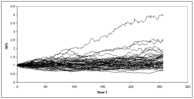
Plot of 50 possible scenarios with a GBM(m=0.001, s= 0.02) model with starting value of 1.
Mean reversion, discussed next, is a modification to GBM that progressively encourages the series to move back towards a mean the further it strays away. Jump Diffusion, discussed after that, acknowledges that there may be shocks to the variable resulting in large discrete jumps. ModelRisk has functions for fitting and projecting GBM and GBM + Mean Reversion and/or Jump Diffusion. The functions work with both returns r and stock prices S.
GBM with mean reversion
The long-run time-series properties of equity prices (amongst other variables) is, of course, of particular interest to financial analysts. There is a strong interest in determining whether stock prices can be characterised as random walk or mean reverting processes because this has an important effect on an asset's value. A stock price follows a mean reverting process if it has a tendency to return to some average value over time, which means that investors may be able to forecast future returns better by using information on past returns to determine the level of reversion to the long-term trend path. A random walk has no memory, which means that any large move in a stock price following a random walk process is permanent and there is no tendency for the price level to return to a trend path over time. The random walk property also implies that the volatility of stock price can grow without bound in the long run: increased volatility lowers a stock's value, so a reduction in volatility due to mean reversion would increase a stock's value.
For a variable x following a Brownian motion random walk, we have the SDE encountered before:

For mean reversion this equation can be modified as follows:

where a > 0 is the speed of reversion. The effect of the dt coefficient is to produce an expectation of moving downwards if x is currently above m and vice versa. Mean reversion models are produced in terms of S or r:

known as the Ornstein-Uhlenbeck process, and this was one of the first models used to describe short term interest rates where it is called the Vasicek model. The problem with the equation is that we can get negative stock prices; modelling in terms of r however:

keeps the stock price positive. Integrating this last equation over time gives:

which is very easy to simulate. The plots on the right show some typical behaviour for rt. Typical values of a would be in the range of 0.1 to 0.3.
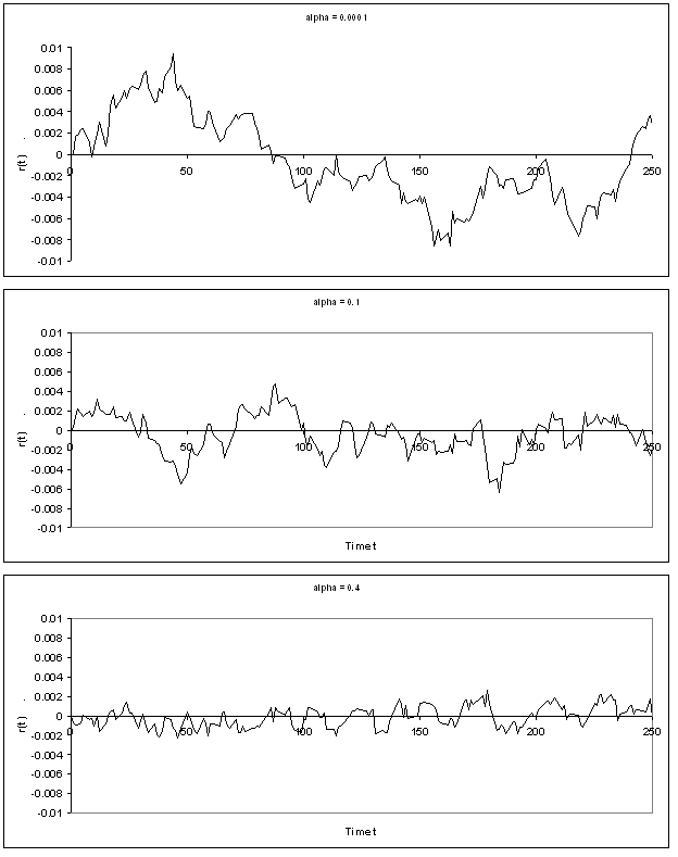
Plots of sample GBM series with mean reversion for different values of alpha (m = 0, s = 0.001)
A slight modification to this is called the Cox-Ingersoll-Ross or CIR model (Cox et al, 1985), again used for short-term interest rates, and has the useful property of not allowing negative values (so we can use it to model the variable S) because the volatility goes to zero as S approaches zero:

Integrating over time we get:

where 
and Y is a non-central Chi-Squared distribution with  degrees of freedom and non-centrality parameter
  . This is a little harder to simulate since you need the uncommon non-central Chi-squared distribution in your simulation software, but it has the attraction of being tractable (we can precisely determine the form of the distribution for the variable St+T) which makes it easier to determine its parameters using maximum likelihood methods.
GBM with jump diffusion
Jump diffusion refers to sudden shocks to the variable that occur randomly in time. The idea is to recognise that beyond the usual background randomness of a time series variable there will be events that have a much larger impact on the variable, e.g. a CEO resigns, a terrorist attack takes place, a drug gets FDA approval. The frequency of the jumps is usually modelled as a Poisson distribution with intensity l so that in some time increment T there will be Poisson(lT) jumps. The jump size for r is usually modelled as Normal(mJ, sJ) for mathematical convenience and ease of estimating the parameters. Adding jump diffusion to the discrete time GBM equation for one period we get the following:

If we define k = Poisson(l), this reduces to:

or for T periods we have:

which is easy to model with Monte Carlo simulation and easy to estimate parameters for by matching moments, although one must be careful to ensure that the l estimate isn't too high (e.g. > 0.2) because the Poisson jumps are meant to be rare events, not form part of each period's volatility. The following plot shows a typical jump diffusion model giving both r and S values and with jumps marked as circles:
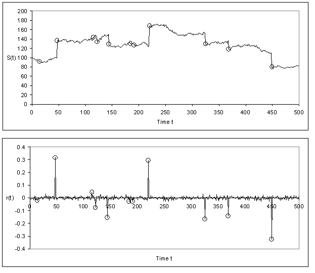
Sample of a GBM with Jump Diffusion with parameters m = 0, s = 0.01, mJ = 0.04, sJ = 0.2, and l = 0.02.
GBM with jump diffusion and mean reversion
You can imagine that if the return r has just received a large shock there might well be a 'correction' over time which brings it back to the expected return m of the series. Combining mean reversion with jump diffusion will allow us to model these characteristics quite well and with few parameters. However, the GBM with jump diffusion model
for mean and variance no longer applies, particularly when the reversion speed is large because one needs to model when within the period the jump took place: if it was at the beginning of the period, it may well have already strongly reverted before one observes the value at the period's end.
The most practical solution, called Euler's method, is to split up a time period into many small increments. The number of increments will be sufficient when the model produces the same output for decision purposes as any greater number of increments.
ModelRisk implements the GBM with both jump diffusion and mean reversion in the VoseTimeGBMJDMR function.
Read on: Autoregressive models
Navigation
- Risk management
- Risk management introduction
- What are risks and opportunities?
- Planning a risk analysis
- Clearly stating risk management questions
- Evaluating risk management options
- Introduction to risk analysis
- The quality of a risk analysis
- Using risk analysis to make better decisions
- Explaining a models assumptions
- Statistical descriptions of model outputs
- Simulation Statistical Results
- Preparing a risk analysis report
- Graphical descriptions of model outputs
- Presenting and using results introduction
- Statistical descriptions of model results
- Mean deviation (MD)
- Range
- Semi-variance and semi-standard deviation
- Kurtosis (K)
- Mean
- Skewness (S)
- Conditional mean
- Custom simulation statistics table
- Mode
- Cumulative percentiles
- Median
- Relative positioning of mode median and mean
- Variance
- Standard deviation
- Inter-percentile range
- Normalized measures of spread - the CofV
- Graphical descriptionss of model results
- Showing probability ranges
- Overlaying histogram plots
- Scatter plots
- Effect of varying number of bars
- Sturges rule
- Relationship between cdf and density (histogram) plots
- Difficulty of interpreting the vertical scale
- Stochastic dominance tests
- Risk-return plots
- Second order cumulative probability plot
- Ascending and descending cumulative plots
- Tornado plot
- Box Plot
- Cumulative distribution function (cdf)
- Probability density function (pdf)
- Crude sensitivity analysis for identifying important input distributions
- Pareto Plot
- Trend plot
- Probability mass function (pmf)
- Overlaying cdf plots
- Cumulative Plot
- Simulation data table
- Statistics table
- Histogram Plot
- Spider plot
- Determining the width of histogram bars
- Plotting a variable with discrete and continuous elements
- Smoothing a histogram plot
- Risk analysis modeling techniques
- Monte Carlo simulation
- Monte Carlo simulation introduction
- Monte Carlo simulation in ModelRisk
- Filtering simulation results
- Output/Input Window
- Simulation Progress control
- Running multiple simulations
- Random number generation in ModelRisk
- Random sampling from input distributions
- How many Monte Carlo samples are enough?
- Probability distributions
- Distributions introduction
- Probability calculations in ModelRisk
- Selecting the appropriate distributions for your model
- List of distributions by category
- Distribution functions and the U parameter
- Univariate continuous distributions
- Beta distribution
- Beta Subjective distribution
- Four-parameter Beta distribution
- Bradford distribution
- Burr distribution
- Cauchy distribution
- Chi distribution
- Chi Squared distribution
- Continuous distributions introduction
- Continuous fitted distribution
- Cumulative ascending distribution
- Cumulative descending distribution
- Dagum distribution
- Erlang distribution
- Error distribution
- Error function distribution
- Exponential distribution
- Exponential family of distributions
- Extreme Value Minimum distribution
- Extreme Value Maximum distribution
- F distribution
- Fatigue Life distribution
- Gamma distribution
- Generalized Extreme Value distribution
- Generalized Logistic distribution
- Generalized Trapezoid Uniform (GTU) distribution
- Histogram distribution
- Hyperbolic-Secant distribution
- Inverse Gaussian distribution
- Johnson Bounded distribution
- Johnson Unbounded distribution
- Kernel Continuous Unbounded distribution
- Kumaraswamy distribution
- Kumaraswamy Four-parameter distribution
- Laplace distribution
- Levy distribution
- Lifetime Two-Parameter distribution
- Lifetime Three-Parameter distribution
- Lifetime Exponential distribution
- LogGamma distribution
- Logistic distribution
- LogLaplace distribution
- LogLogistic distribution
- LogLogistic Alternative parameter distribution
- LogNormal distribution
- LogNormal Alternative-parameter distribution
- LogNormal base B distribution
- LogNormal base E distribution
- LogTriangle distribution
- LogUniform distribution
- Noncentral Chi squared distribution
- Noncentral F distribution
- Normal distribution
- Normal distribution with alternative parameters
- Maxwell distribution
- Normal Mix distribution
- Relative distribution
- Ogive distribution
- Pareto (first kind) distribution
- Pareto (second kind) distribution
- Pearson Type 5 distribution
- Pearson Type 6 distribution
- Modified PERT distribution
- PERT distribution
- PERT Alternative-parameter distribution
- Reciprocal distribution
- Rayleigh distribution
- Skew Normal distribution
- Slash distribution
- SplitTriangle distribution
- Student-t distribution
- Three-parameter Student distribution
- Triangle distribution
- Triangle Alternative-parameter distribution
- Uniform distribution
- Weibull distribution
- Weibull Alternative-parameter distribution
- Three-Parameter Weibull distribution
- Univariate discrete distributions
- Discrete distributions introduction
- Bernoulli distribution
- Beta-Binomial distribution
- Beta-Geometric distribution
- Beta-Negative Binomial distribution
- Binomial distribution
- Burnt Finger Poisson distribution
- Delaporte distribution
- Discrete distribution
- Discrete Fitted distribution
- Discrete Uniform distribution
- Geometric distribution
- HypergeoM distribution
- Hypergeometric distribution
- HypergeoD distribution
- Inverse Hypergeometric distribution
- Logarithmic distribution
- Negative Binomial distribution
- Poisson distribution
- Poisson Uniform distribution
- Polya distribution
- Skellam distribution
- Step Uniform distribution
- Zero-modified counting distributions
- More on probability distributions
- Multivariate distributions
- Multivariate distributions introduction
- Dirichlet distribution
- Multinomial distribution
- Multivariate Hypergeometric distribution
- Multivariate Inverse Hypergeometric distribution type2
- Negative Multinomial distribution type 1
- Negative Multinomial distribution type 2
- Multivariate Inverse Hypergeometric distribution type1
- Multivariate Normal distribution
- More on probability distributions
- Approximating one distribution with another
- Approximations to the Inverse Hypergeometric Distribution
- Normal approximation to the Gamma Distribution
- Normal approximation to the Poisson Distribution
- Approximations to the Hypergeometric Distribution
- Stirlings formula for factorials
- Normal approximation to the Beta Distribution
- Approximation of one distribution with another
- Approximations to the Negative Binomial Distribution
- Normal approximation to the Student-t Distribution
- Approximations to the Binomial Distribution
- Normal_approximation_to_the_Binomial_distribution
- Poisson_approximation_to_the_Binomial_distribution
- Normal approximation to the Chi Squared Distribution
- Recursive formulas for discrete distributions
- Normal approximation to the Lognormal Distribution
- Normal approximations to other distributions
- Approximating one distribution with another
- Correlation modeling in risk analysis
- Common mistakes when adapting spreadsheet models for risk analysis
- More advanced risk analysis methods
- SIDs
- Modeling with objects
- ModelRisk database connectivity functions
- PK/PD modeling
- Value of information techniques
- Simulating with ordinary differential equations (ODEs)
- Optimization of stochastic models
- ModelRisk optimization extension introduction
- Optimization Settings
- Defining Simulation Requirements in an Optimization Model
- Defining Decision Constraints in an Optimization Model
- Optimization Progress control
- Defining Targets in an Optimization Model
- Defining Decision Variables in an Optimization Model
- Optimization Results
- Summing random variables
- Aggregate distributions introduction
- Aggregate modeling - Panjer's recursive method
- Adding correlation in aggregate calculations
- Sum of a random number of random variables
- Moments of an aggregate distribution
- Aggregate modeling in ModelRisk
- Aggregate modeling - Fast Fourier Transform (FFT) method
- How many random variables add up to a fixed total
- Aggregate modeling - compound Poisson approximation
- Aggregate modeling - De Pril's recursive method
- Testing and modeling causal relationships
- Stochastic time series
- Time series introduction
- Time series in ModelRisk
- Autoregressive models
- Thiel inequality coefficient
- Effect of an intervention at some uncertain point in time
- Log return of a Time Series
- Markov Chain models
- Seasonal time series
- Bounded random walk
- Time series modeling in finance
- Birth and death models
- Time series models with leading indicators
- Geometric Brownian Motion models
- Time series projection of events occurring randomly in time
- Simulation for six sigma
- ModelRisk's Six Sigma functions
- VoseSixSigmaCp
- VoseSixSigmaCpkLower
- VoseSixSigmaProbDefectShift
- VoseSixSigmaLowerBound
- VoseSixSigmaK
- VoseSixSigmaDefectShiftPPMUpper
- VoseSixSigmaDefectShiftPPMLower
- VoseSixSigmaDefectShiftPPM
- VoseSixSigmaCpm
- VoseSixSigmaSigmaLevel
- VoseSixSigmaCpkUpper
- VoseSixSigmaCpk
- VoseSixSigmaDefectPPM
- VoseSixSigmaProbDefectShiftLower
- VoseSixSigmaProbDefectShiftUpper
- VoseSixSigmaYield
- VoseSixSigmaUpperBound
- VoseSixSigmaZupper
- VoseSixSigmaZmin
- VoseSixSigmaZlower
- Modeling expert opinion
- Modeling expert opinion introduction
- Sources of error in subjective estimation
- Disaggregation
- Distributions used in modeling expert opinion
- A subjective estimate of a discrete quantity
- Incorporating differences in expert opinions
- Modeling opinion of a variable that covers several orders of magnitude
- Maximum entropy
- Probability theory and statistics
- Probability theory and statistics introduction
- Stochastic processes
- Stochastic processes introduction
- Poisson process
- Hypergeometric process
- The hypergeometric process
- Number in a sample with a particular characteristic in a hypergeometric process
- Number of hypergeometric samples to get a specific number of successes
- Number of samples taken to have an observed s in a hypergeometric process
- Estimate of population and sub-population sizes in a hypergeometric process
- The binomial process
- Renewal processes
- Mixture processes
- Martingales
- Estimating model parameters from data
- The basics
- Probability equations
- Probability theorems and useful concepts
- Probability parameters
- Probability rules and diagrams
- The definition of probability
- The basics of probability theory introduction
- Fitting probability models to data
- Fitting time series models to data
- Fitting correlation structures to data
- Fitting in ModelRisk
- Fitting probability distributions to data
- Fitting distributions to data
- Method of Moments (MoM)
- Check the quality of your data
- Kolmogorov-Smirnoff (K-S) Statistic
- Anderson-Darling (A-D) Statistic
- Goodness of fit statistics
- The Chi-Squared Goodness-of-Fit Statistic
- Determining the joint uncertainty distribution for parameters of a distribution
- Using Method of Moments with the Bootstrap
- Maximum Likelihood Estimates (MLEs)
- Fitting a distribution to truncated censored or binned data
- Critical Values and Confidence Intervals for Goodness-of-Fit Statistics
- Matching the properties of the variable and distribution
- Transforming discrete data before performing a parametric distribution fit
- Does a parametric distribution exist that is well known to fit this type of variable?
- Censored data
- Fitting a continuous non-parametric second-order distribution to data
- Goodness of Fit Plots
- Fitting a second order Normal distribution to data
- Using Goodness-of Fit Statistics to optimize Distribution Fitting
- Information criteria - SIC HQIC and AIC
- Fitting a second order parametric distribution to observed data
- Fitting a distribution for a continuous variable
- Does the random variable follow a stochastic process with a well-known model?
- Fitting a distribution for a discrete variable
- Fitting a discrete non-parametric second-order distribution to data
- Fitting a continuous non-parametric first-order distribution to data
- Fitting a first order parametric distribution to observed data
- Fitting a discrete non-parametric first-order distribution to data
- Fitting distributions to data
- Technical subjects
- Comparison of Classical and Bayesian methods
- Comparison of classic and Bayesian estimate of Normal distribution parameters
- Comparison of classic and Bayesian estimate of intensity lambda in a Poisson process
- Comparison of classic and Bayesian estimate of probability p in a binomial process
- Which technique should you use?
- Comparison of classic and Bayesian estimate of mean "time" beta in a Poisson process
- Classical statistics
- Bayesian
- Bootstrap
- The Bootstrap
- Linear regression parametric Bootstrap
- The Jackknife
- Multiple variables Bootstrap Example 2: Difference between two population means
- Linear regression non-parametric Bootstrap
- The parametric Bootstrap
- Bootstrap estimate of prevalence
- Estimating parameters for multiple variables
- Example: Parametric Bootstrap estimate of the mean of a Normal distribution with known standard deviation
- The non-parametric Bootstrap
- Example: Parametric Bootstrap estimate of mean number of calls per hour at a telephone exchange
- The Bootstrap likelihood function for Bayesian inference
- Multiple variables Bootstrap Example 1: Estimate of regression parameters
- Bayesian inference
- Uninformed priors
- Conjugate priors
- Prior distributions
- Bayesian analysis with threshold data
- Bayesian analysis example: gender of a random sample of people
- Informed prior
- Simulating a Bayesian inference calculation
- Hyperparameters
- Hyperparameter example: Micro-fractures on turbine blades
- Constructing a Bayesian inference posterior distribution in Excel
- Bayesian analysis example: Tigers in the jungle
- Markov chain Monte Carlo (MCMC) simulation
- Introduction to Bayesian inference concepts
- Bayesian estimate of the mean of a Normal distribution with known standard deviation
- Bayesian estimate of the mean of a Normal distribution with unknown standard deviation
- Determining prior distributions for correlated parameters
- Improper priors
- The Jacobian transformation
- Subjective prior based on data
- Taylor series approximation to a Bayesian posterior distribution
- Bayesian analysis example: The Monty Hall problem
- Determining prior distributions for uncorrelated parameters
- Subjective priors
- Normal approximation to the Beta posterior distribution
- Bayesian analysis example: identifying a weighted coin
- Bayesian estimate of the standard deviation of a Normal distribution with known mean
- Likelihood functions
- Bayesian estimate of the standard deviation of a Normal distribution with unknown mean
- Determining a prior distribution for a single parameter estimate
- Simulating from a constructed posterior distribution
- Bootstrap
- Comparison of Classical and Bayesian methods
- Analyzing and using data introduction
- Data Object
- Vose probability calculation
- Bayesian model averaging
- Miscellaneous
- Excel and ModelRisk model design and validation techniques
- Using range names for model clarity
- Color coding models for clarity
- Compare with known answers
- Checking units propagate correctly
- Stressing parameter values
- Model Validation and behavior introduction
- Informal auditing
- Analyzing outputs
- View random scenarios on screen and check for credibility
- Split up complex formulas (megaformulas)
- Building models that are efficient
- Comparing predictions against reality
- Numerical integration
- Comparing results of alternative models
- Building models that are easy to check and modify
- Model errors
- Model design introduction
- About array functions in Excel
- Excel and ModelRisk model design and validation techniques
- Monte Carlo simulation
- RISK ANALYSIS SOFTWARE
- Risk analysis software from Vose Software
- ModelRisk - risk modeling in Excel
- ModelRisk functions explained
- VoseCopulaOptimalFit and related functions
- VoseTimeOptimalFit and related functions
- VoseOptimalFit and related functions
- VoseXBounds
- VoseCLTSum
- VoseAggregateMoments
- VoseRawMoments
- VoseSkewness
- VoseMoments
- VoseKurtosis
- VoseAggregatePanjer
- VoseAggregateFFT
- VoseCombined
- VoseCopulaBiGumbel
- VoseCopulaBiClayton
- VoseCopulaBiNormal
- VoseCopulaBiT
- VoseKendallsTau
- VoseRiskEvent
- VoseCopulaBiFrank
- VoseCorrMatrix
- VoseRank
- VoseValidCorrmat
- VoseSpearman
- VoseCopulaData
- VoseCorrMatrixU
- VoseTimeSeasonalGBM
- VoseMarkovSample
- VoseMarkovMatrix
- VoseThielU
- VoseTimeEGARCH
- VoseTimeAPARCH
- VoseTimeARMA
- VoseTimeDeath
- VoseTimeAR1
- VoseTimeAR2
- VoseTimeARCH
- VoseTimeMA2
- VoseTimeGARCH
- VoseTimeGBMJDMR
- VoseTimePriceInflation
- VoseTimeGBMMR
- VoseTimeWageInflation
- VoseTimeLongTermInterestRate
- VoseTimeMA1
- VoseTimeGBM
- VoseTimeGBMJD
- VoseTimeShareYields
- VoseTimeYule
- VoseTimeShortTermInterestRate
- VoseDominance
- VoseLargest
- VoseSmallest
- VoseShift
- VoseStopSum
- VoseEigenValues
- VosePrincipleEsscher
- VoseAggregateMultiFFT
- VosePrincipleEV
- VoseCopulaMultiNormal
- VoseRunoff
- VosePrincipleRA
- VoseSumProduct
- VosePrincipleStdev
- VosePoissonLambda
- VoseBinomialP
- VosePBounds
- VoseAIC
- VoseHQIC
- VoseSIC
- VoseOgive1
- VoseFrequency
- VoseOgive2
- VoseNBootStdev
- VoseNBoot
- VoseSimulate
- VoseNBootPaired
- VoseAggregateMC
- VoseMean
- VoseStDev
- VoseAggregateMultiMoments
- VoseDeduct
- VoseExpression
- VoseLargestSet
- VoseKthSmallest
- VoseSmallestSet
- VoseKthLargest
- VoseNBootCofV
- VoseNBootPercentile
- VoseExtremeRange
- VoseNBootKurt
- VoseCopulaMultiClayton
- VoseNBootMean
- VoseTangentPortfolio
- VoseNBootVariance
- VoseNBootSkewness
- VoseIntegrate
- VoseInterpolate
- VoseCopulaMultiGumbel
- VoseCopulaMultiT
- VoseAggregateMultiMC
- VoseCopulaMultiFrank
- VoseTimeMultiMA1
- VoseTimeMultiMA2
- VoseTimeMultiGBM
- VoseTimeMultBEKK
- VoseAggregateDePril
- VoseTimeMultiAR1
- VoseTimeWilkie
- VoseTimeDividends
- VoseTimeMultiAR2
- VoseRuinFlag
- VoseRuinTime
- VoseDepletionShortfall
- VoseDepletion
- VoseDepletionFlag
- VoseDepletionTime
- VosejProduct
- VoseCholesky
- VoseTimeSimulate
- VoseNBootSeries
- VosejkProduct
- VoseRuinSeverity
- VoseRuin
- VosejkSum
- VoseTimeDividendsA
- VoseRuinNPV
- VoseTruncData
- VoseSample
- VoseIdentity
- VoseCopulaSimulate
- VoseSortA
- VoseFrequencyCumulA
- VoseAggregateDeduct
- VoseMeanExcessP
- VoseProb10
- VoseSpearmanU
- VoseSortD
- VoseFrequencyCumulD
- VoseRuinMaxSeverity
- VoseMeanExcessX
- VoseRawMoment3
- VosejSum
- VoseRawMoment4
- VoseNBootMoments
- VoseVariance
- VoseTimeShortTermInterestRateA
- VoseTimeLongTermInterestRateA
- VoseProb
- VoseDescription
- VoseCofV
- VoseAggregateProduct
- VoseEigenVectors
- VoseTimeWageInflationA
- VoseRawMoment1
- VosejSumInf
- VoseRawMoment2
- VoseShuffle
- VoseRollingStats
- VoseSplice
- VoseTSEmpiricalFit
- VoseTimeShareYieldsA
- VoseParameters
- VoseAggregateTranche
- VoseCovToCorr
- VoseCorrToCov
- VoseLLH
- VoseTimeSMEThreePoint
- VoseDataObject
- VoseCopulaDataSeries
- VoseDataRow
- VoseDataMin
- VoseDataMax
- VoseTimeSME2Perc
- VoseTimeSMEUniform
- VoseTimeSMESaturation
- VoseOutput
- VoseInput
- VoseTimeSMEPoisson
- VoseTimeBMAObject
- VoseBMAObject
- VoseBMAProb10
- VoseBMAProb
- VoseCopulaBMA
- VoseCopulaBMAObject
- VoseTimeEmpiricalFit
- VoseTimeBMA
- VoseBMA
- VoseSimKurtosis
- VoseOptConstraintMin
- VoseSimProbability
- VoseCurrentSample
- VoseCurrentSim
- VoseLibAssumption
- VoseLibReference
- VoseSimMoments
- VoseOptConstraintMax
- VoseSimMean
- VoseOptDecisionContinuous
- VoseOptRequirementEquals
- VoseOptRequirementMax
- VoseOptRequirementMin
- VoseOptTargetMinimize
- VoseOptConstraintEquals
- VoseSimVariance
- VoseSimSkewness
- VoseSimTable
- VoseSimCofV
- VoseSimPercentile
- VoseSimStDev
- VoseOptTargetValue
- VoseOptTargetMaximize
- VoseOptDecisionDiscrete
- VoseSimMSE
- VoseMin
- VoseMin
- VoseOptDecisionList
- VoseOptDecisionBoolean
- VoseOptRequirementBetween
- VoseOptConstraintBetween
- VoseSimMax
- VoseSimSemiVariance
- VoseSimSemiStdev
- VoseSimMeanDeviation
- VoseSimMin
- VoseSimCVARp
- VoseSimCVARx
- VoseSimCorrelation
- VoseSimCorrelationMatrix
- VoseOptConstraintString
- VoseOptCVARx
- VoseOptCVARp
- VoseOptPercentile
- VoseSimValue
- VoseSimStop
- Precision Control Functions
- VoseAggregateDiscrete
- VoseTimeMultiGARCH
- VoseTimeGBMVR
- VoseTimeGBMAJ
- VoseTimeGBMAJVR
- VoseSID
- Generalized Pareto Distribution (GPD)
- Generalized Pareto Distribution (GPD) Equations
- Three-Point Estimate Distribution
- Three-Point Estimate Distribution Equations
- VoseCalibrate
- ModelRisk interfaces
- Integrate
- Data Viewer
- Stochastic Dominance
- Library
- Correlation Matrix
- Portfolio Optimization Model
- Common elements of ModelRisk interfaces
- Risk Event
- Extreme Values
- Select Distribution
- Combined Distribution
- Aggregate Panjer
- Interpolate
- View Function
- Find Function
- Deduct
- Ogive
- AtRISK model converter
- Aggregate Multi FFT
- Stop Sum
- Crystal Ball model converter
- Aggregate Monte Carlo
- Splicing Distributions
- Subject Matter Expert (SME) Time Series Forecasts
- Aggregate Multivariate Monte Carlo
- Ordinary Differential Equation tool
- Aggregate FFT
- More on Conversion
- Multivariate Copula
- Bivariate Copula
- Univariate Time Series
- Modeling expert opinion in ModelRisk
- Multivariate Time Series
- Sum Product
- Aggregate DePril
- Aggregate Discrete
- Expert
- ModelRisk introduction
- Building and running a simple example model
- Distributions in ModelRisk
- List of all ModelRisk functions
- Custom applications and macros
- ModelRisk functions explained
- Tamara - project risk analysis
- Introduction to Tamara project risk analysis software
- Launching Tamara
- Importing a schedule
- Assigning uncertainty to the amount of work in the project
- Assigning uncertainty to productivity levels in the project
- Adding risk events to the project schedule
- Adding cost uncertainty to the project schedule
- Saving the Tamara model
- Running a Monte Carlo simulation in Tamara
- Reviewing the simulation results in Tamara
- Using Tamara results for cost and financial risk analysis
- Creating, updating and distributing a Tamara report
- Tips for creating a schedule model suitable for Monte Carlo simulation
- Random number generator and sampling algorithms used in Tamara
- Probability distributions used in Tamara
- Correlation with project schedule risk analysis
- Pelican - enterprise risk management