Common elements of ModelRisk windows
See also: ModelRisk functions and windows, Statistical descriptions of model outputs, Graphical descriptions of model outputs, Graphics, workflow and error handling in ModelRisk
Quickly jump to:
- Common fields and buttons
- Summary statistics table
- Preview graphs
- Errors
Certain elements appear in many ModelRisk windows. For example, a table with summary statistics; graphs; and fields like the output field.
This topic gives a more in-depth explanation about these elements and how to use them.
Fields and buttons - Output location, M/C, Generate, Help, OK, Cancel
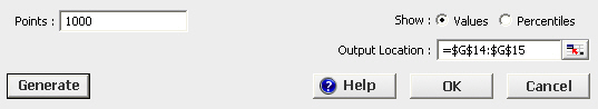
Most of the ModelRisk windows correspond to a VoseFunction (e.g. an aggregate distribution, sampled value from a spliced distribution, etc...) being inserted in one or more spreadsheet cells. The location where the VoseFunction is to be inserted in the spreadsheet, is specified in the Output Location field. The desired VoseFunction will be inserted upon pressing the OK button, after which the ModelRisk window closes.
 Pressing the Cancel button closes the window without modifying the spreadsheet in any way. Pressing the Esc keyboard button has the same effect.
The Generate button re-generates the random values for the preview graph(s) in the window.
With the M and C buttons you can switch between viewing the Probability Density (or Mass), or cumulative graphs of the distribution(s) shown.

Summary statistics table
 Distributions and their properties play a central role in risk analysis modeling.
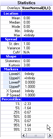
In all ModelRisk windows that have a function related to distributions (which many do), a table with summary statistics of the currently selected/loaded/previewed distribution is shown on the right. For ease of use, this table always contains the same elements, regardless of the specific ModelRisk window it is in. These elements are:
Location
- Mean
- Median
- Mode
- Min
- Max
Spread
- Standard deviation (St. dev.)
- Variance
- Coefficient of Variation (CofV)
Shape
- Skewness (S)
- Kurtosis (K)
Where it is relevant, the following statistics are shown as well:
Markers
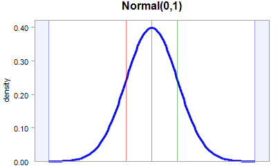
Markers can be edited in the statistics pane. Use markers to see the x-values corresponding to percentiles, and vice versa. For example, the image shows what you see when setting the LowerX value to -1 and the UpperX value to 1 for a normal(0,1):
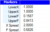
- LowerX - the lower marker value (-infinity by default)
- UpperX - the Upper marker value (+infinity by default)
- LowerP - the Lower marker's Percentile value (0 by default)
- UpperP - the Upper marker's Percentile value (1 by default)
- X Spread - the range between the markers, i.e. UpperX - LowerX
- P Spread - the percentile range between the markers, i.e. UpperP - LowerP
The marker settings shown in the image correspond to this PDF plot:
Percentiles
The 1st, 5th, 25th, 50th, 75th, 95th and 99th percentiles are always shown. If the ModelRisk window is enlarged (by dragging its lower right corner), additional percentiles are shown.
Preview graphs
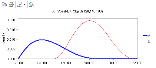 In windows where distributions play a role, the PDF or PMF, CDF or both graphs are shown.
When you hold the mouse pointer above a graph, it comes "in focus" and all other visible elements are greyed out, for easily pointing somebody to a certain graph.
The graphs update dynamically according to the distribution's parameter values when these can be specified within the window.
On top of graphs are the graph toolbar buttons. Below is explained what you can do with the most important of these buttons. Note that these buttons are not necessarily all present in a given ModelRisk window.
-
 Copy to clipboard, either as a bitmap, metafile or text (data only). This allows you to use the graph image in other programs, like MS PowerPoint, or for your web site... (try copying as bitmap, and then pasting in MS Paint by pressing CTRL+V)
- To copy the image as you see it presented, including colors etc... choose As a bitmap. This is the "normal" way to copy an image to the clipboard, like you are probably used to doing in Windows.
- You can also copy the image to the clipboard as a metafile (WMF), the Windows vector file format. An advantage of vector graphics is that they can be rescaled without quality loss (in the proper program). Most fonts in Windows are basically vector graphics, for example.
- You can also copy the (randomly sampled) source data, used to construct the preview graphs, as text to the clipboard. For a PDF graph this is a set of (x,y) pairs, for example.

Export options in the Empirical Copula window
-
 Print. This will take you to the common Windows dialog for selecting a printer, adjusting printing options, and of course print the graph(s).
 -
 Palette Selector. You can adjust the graphs colors to one of the preset color palettes. Note that every graph element can be formatted individually as well by right-clicking it.
 -
 Zoom. To zoom in to a part of the plot, press the Zoom button and then drag a rectangle in the graph area. This will zoom in to this graph. To zoom out again, press the Zoom button again.
 -
 Edit X axis. This allows you to set the boundaries shown for the X-axis, or to toggle "auto scale mode" (to scale the X axis automatically).
 -
 Properties. Change more properties of the graph, like colors of every element, font formatting, 3D view...
 -
 Export options. Whenever a ModelRisk window has more than one type of output to insert in the spreadsheet, these Window-specific types of output can be accessed with the Export options button above the preview graph.
Industrial version only
-
 Create report. Clicking this button will produce a fit report in a new Worksheet with the fitted models in a table. The table will have the fitted objects, rankings, statistics and percentiles of the fitted models. (This depends on object type) The report will also include the OptimatFit function that automatically returns the best fitted model according to the selected information criteria.
Whenever a preview graph has boundaries (visualized by vertical lines), these can be dragged along the graph to change the corresponding boundary value.
By right-clicking anywhere in the graph area, you can quickly access many of the above through the context menu that pops up.
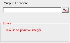
Errors
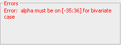 In ModelRisk windows, a descriptive error message is shown in red when appropriate. For example, the bivariate copula requires an Alpha parameter between -35 and 36. If the currently chosen Alpha lies outside of this range, this will be pointed out in red. For more information about errors in ModelRisk, click here.
For general troubleshooting, also see the FAQ - Troubleshooting topic.
Navigation
- Risk management
- Risk management introduction
- What are risks and opportunities?
- Planning a risk analysis
- Clearly stating risk management questions
- Evaluating risk management options
- Introduction to risk analysis
- The quality of a risk analysis
- Using risk analysis to make better decisions
- Explaining a models assumptions
- Statistical descriptions of model outputs
- Simulation Statistical Results
- Preparing a risk analysis report
- Graphical descriptions of model outputs
- Presenting and using results introduction
- Statistical descriptions of model results
- Mean deviation (MD)
- Range
- Semi-variance and semi-standard deviation
- Kurtosis (K)
- Mean
- Skewness (S)
- Conditional mean
- Custom simulation statistics table
- Mode
- Cumulative percentiles
- Median
- Relative positioning of mode median and mean
- Variance
- Standard deviation
- Inter-percentile range
- Normalized measures of spread - the CofV
- Graphical descriptionss of model results
- Showing probability ranges
- Overlaying histogram plots
- Scatter plots
- Effect of varying number of bars
- Sturges rule
- Relationship between cdf and density (histogram) plots
- Difficulty of interpreting the vertical scale
- Stochastic dominance tests
- Risk-return plots
- Second order cumulative probability plot
- Ascending and descending cumulative plots
- Tornado plot
- Box Plot
- Cumulative distribution function (cdf)
- Probability density function (pdf)
- Crude sensitivity analysis for identifying important input distributions
- Pareto Plot
- Trend plot
- Probability mass function (pmf)
- Overlaying cdf plots
- Cumulative Plot
- Simulation data table
- Statistics table
- Histogram Plot
- Spider plot
- Determining the width of histogram bars
- Plotting a variable with discrete and continuous elements
- Smoothing a histogram plot
- Risk analysis modeling techniques
- Monte Carlo simulation
- Monte Carlo simulation introduction
- Monte Carlo simulation in ModelRisk
- Filtering simulation results
- Output/Input Window
- Simulation Progress control
- Running multiple simulations
- Random number generation in ModelRisk
- Random sampling from input distributions
- How many Monte Carlo samples are enough?
- Probability distributions
- Distributions introduction
- Probability calculations in ModelRisk
- Selecting the appropriate distributions for your model
- List of distributions by category
- Distribution functions and the U parameter
- Univariate continuous distributions
- Beta distribution
- Beta Subjective distribution
- Four-parameter Beta distribution
- Bradford distribution
- Burr distribution
- Cauchy distribution
- Chi distribution
- Chi Squared distribution
- Continuous distributions introduction
- Continuous fitted distribution
- Cumulative ascending distribution
- Cumulative descending distribution
- Dagum distribution
- Erlang distribution
- Error distribution
- Error function distribution
- Exponential distribution
- Exponential family of distributions
- Extreme Value Minimum distribution
- Extreme Value Maximum distribution
- F distribution
- Fatigue Life distribution
- Gamma distribution
- Generalized Extreme Value distribution
- Generalized Logistic distribution
- Generalized Trapezoid Uniform (GTU) distribution
- Histogram distribution
- Hyperbolic-Secant distribution
- Inverse Gaussian distribution
- Johnson Bounded distribution
- Johnson Unbounded distribution
- Kernel Continuous Unbounded distribution
- Kumaraswamy distribution
- Kumaraswamy Four-parameter distribution
- Laplace distribution
- Levy distribution
- Lifetime Two-Parameter distribution
- Lifetime Three-Parameter distribution
- Lifetime Exponential distribution
- LogGamma distribution
- Logistic distribution
- LogLaplace distribution
- LogLogistic distribution
- LogLogistic Alternative parameter distribution
- LogNormal distribution
- LogNormal Alternative-parameter distribution
- LogNormal base B distribution
- LogNormal base E distribution
- LogTriangle distribution
- LogUniform distribution
- Noncentral Chi squared distribution
- Noncentral F distribution
- Normal distribution
- Normal distribution with alternative parameters
- Maxwell distribution
- Normal Mix distribution
- Relative distribution
- Ogive distribution
- Pareto (first kind) distribution
- Pareto (second kind) distribution
- Pearson Type 5 distribution
- Pearson Type 6 distribution
- Modified PERT distribution
- PERT distribution
- PERT Alternative-parameter distribution
- Reciprocal distribution
- Rayleigh distribution
- Skew Normal distribution
- Slash distribution
- SplitTriangle distribution
- Student-t distribution
- Three-parameter Student distribution
- Triangle distribution
- Triangle Alternative-parameter distribution
- Uniform distribution
- Weibull distribution
- Weibull Alternative-parameter distribution
- Three-Parameter Weibull distribution
- Univariate discrete distributions
- Discrete distributions introduction
- Bernoulli distribution
- Beta-Binomial distribution
- Beta-Geometric distribution
- Beta-Negative Binomial distribution
- Binomial distribution
- Burnt Finger Poisson distribution
- Delaporte distribution
- Discrete distribution
- Discrete Fitted distribution
- Discrete Uniform distribution
- Geometric distribution
- HypergeoM distribution
- Hypergeometric distribution
- HypergeoD distribution
- Inverse Hypergeometric distribution
- Logarithmic distribution
- Negative Binomial distribution
- Poisson distribution
- Poisson Uniform distribution
- Polya distribution
- Skellam distribution
- Step Uniform distribution
- Zero-modified counting distributions
- More on probability distributions
- Multivariate distributions
- Multivariate distributions introduction
- Dirichlet distribution
- Multinomial distribution
- Multivariate Hypergeometric distribution
- Multivariate Inverse Hypergeometric distribution type2
- Negative Multinomial distribution type 1
- Negative Multinomial distribution type 2
- Multivariate Inverse Hypergeometric distribution type1
- Multivariate Normal distribution
- More on probability distributions
- Approximating one distribution with another
- Approximations to the Inverse Hypergeometric Distribution
- Normal approximation to the Gamma Distribution
- Normal approximation to the Poisson Distribution
- Approximations to the Hypergeometric Distribution
- Stirlings formula for factorials
- Normal approximation to the Beta Distribution
- Approximation of one distribution with another
- Approximations to the Negative Binomial Distribution
- Normal approximation to the Student-t Distribution
- Approximations to the Binomial Distribution
- Normal_approximation_to_the_Binomial_distribution
- Poisson_approximation_to_the_Binomial_distribution
- Normal approximation to the Chi Squared Distribution
- Recursive formulas for discrete distributions
- Normal approximation to the Lognormal Distribution
- Normal approximations to other distributions
- Approximating one distribution with another
- Correlation modeling in risk analysis
- Common mistakes when adapting spreadsheet models for risk analysis
- More advanced risk analysis methods
- SIDs
- Modeling with objects
- ModelRisk database connectivity functions
- PK/PD modeling
- Value of information techniques
- Simulating with ordinary differential equations (ODEs)
- Optimization of stochastic models
- ModelRisk optimization extension introduction
- Optimization Settings
- Defining Simulation Requirements in an Optimization Model
- Defining Decision Constraints in an Optimization Model
- Optimization Progress control
- Defining Targets in an Optimization Model
- Defining Decision Variables in an Optimization Model
- Optimization Results
- Summing random variables
- Aggregate distributions introduction
- Aggregate modeling - Panjer's recursive method
- Adding correlation in aggregate calculations
- Sum of a random number of random variables
- Moments of an aggregate distribution
- Aggregate modeling in ModelRisk
- Aggregate modeling - Fast Fourier Transform (FFT) method
- How many random variables add up to a fixed total
- Aggregate modeling - compound Poisson approximation
- Aggregate modeling - De Pril's recursive method
- Testing and modeling causal relationships
- Stochastic time series
- Time series introduction
- Time series in ModelRisk
- Autoregressive models
- Thiel inequality coefficient
- Effect of an intervention at some uncertain point in time
- Log return of a Time Series
- Markov Chain models
- Seasonal time series
- Bounded random walk
- Time series modeling in finance
- Birth and death models
- Time series models with leading indicators
- Geometric Brownian Motion models
- Time series projection of events occurring randomly in time
- Simulation for six sigma
- ModelRisk's Six Sigma functions
- VoseSixSigmaCp
- VoseSixSigmaCpkLower
- VoseSixSigmaProbDefectShift
- VoseSixSigmaLowerBound
- VoseSixSigmaK
- VoseSixSigmaDefectShiftPPMUpper
- VoseSixSigmaDefectShiftPPMLower
- VoseSixSigmaDefectShiftPPM
- VoseSixSigmaCpm
- VoseSixSigmaSigmaLevel
- VoseSixSigmaCpkUpper
- VoseSixSigmaCpk
- VoseSixSigmaDefectPPM
- VoseSixSigmaProbDefectShiftLower
- VoseSixSigmaProbDefectShiftUpper
- VoseSixSigmaYield
- VoseSixSigmaUpperBound
- VoseSixSigmaZupper
- VoseSixSigmaZmin
- VoseSixSigmaZlower
- Modeling expert opinion
- Modeling expert opinion introduction
- Sources of error in subjective estimation
- Disaggregation
- Distributions used in modeling expert opinion
- A subjective estimate of a discrete quantity
- Incorporating differences in expert opinions
- Modeling opinion of a variable that covers several orders of magnitude
- Maximum entropy
- Probability theory and statistics
- Probability theory and statistics introduction
- Stochastic processes
- Stochastic processes introduction
- Poisson process
- Hypergeometric process
- The hypergeometric process
- Number in a sample with a particular characteristic in a hypergeometric process
- Number of hypergeometric samples to get a specific number of successes
- Number of samples taken to have an observed s in a hypergeometric process
- Estimate of population and sub-population sizes in a hypergeometric process
- The binomial process
- Renewal processes
- Mixture processes
- Martingales
- Estimating model parameters from data
- The basics
- Probability equations
- Probability theorems and useful concepts
- Probability parameters
- Probability rules and diagrams
- The definition of probability
- The basics of probability theory introduction
- Fitting probability models to data
- Fitting time series models to data
- Fitting correlation structures to data
- Fitting in ModelRisk
- Fitting probability distributions to data
- Fitting distributions to data
- Method of Moments (MoM)
- Check the quality of your data
- Kolmogorov-Smirnoff (K-S) Statistic
- Anderson-Darling (A-D) Statistic
- Goodness of fit statistics
- The Chi-Squared Goodness-of-Fit Statistic
- Determining the joint uncertainty distribution for parameters of a distribution
- Using Method of Moments with the Bootstrap
- Maximum Likelihood Estimates (MLEs)
- Fitting a distribution to truncated censored or binned data
- Critical Values and Confidence Intervals for Goodness-of-Fit Statistics
- Matching the properties of the variable and distribution
- Transforming discrete data before performing a parametric distribution fit
- Does a parametric distribution exist that is well known to fit this type of variable?
- Censored data
- Fitting a continuous non-parametric second-order distribution to data
- Goodness of Fit Plots
- Fitting a second order Normal distribution to data
- Using Goodness-of Fit Statistics to optimize Distribution Fitting
- Information criteria - SIC HQIC and AIC
- Fitting a second order parametric distribution to observed data
- Fitting a distribution for a continuous variable
- Does the random variable follow a stochastic process with a well-known model?
- Fitting a distribution for a discrete variable
- Fitting a discrete non-parametric second-order distribution to data
- Fitting a continuous non-parametric first-order distribution to data
- Fitting a first order parametric distribution to observed data
- Fitting a discrete non-parametric first-order distribution to data
- Fitting distributions to data
- Technical subjects
- Comparison of Classical and Bayesian methods
- Comparison of classic and Bayesian estimate of Normal distribution parameters
- Comparison of classic and Bayesian estimate of intensity lambda in a Poisson process
- Comparison of classic and Bayesian estimate of probability p in a binomial process
- Which technique should you use?
- Comparison of classic and Bayesian estimate of mean "time" beta in a Poisson process
- Classical statistics
- Bayesian
- Bootstrap
- The Bootstrap
- Linear regression parametric Bootstrap
- The Jackknife
- Multiple variables Bootstrap Example 2: Difference between two population means
- Linear regression non-parametric Bootstrap
- The parametric Bootstrap
- Bootstrap estimate of prevalence
- Estimating parameters for multiple variables
- Example: Parametric Bootstrap estimate of the mean of a Normal distribution with known standard deviation
- The non-parametric Bootstrap
- Example: Parametric Bootstrap estimate of mean number of calls per hour at a telephone exchange
- The Bootstrap likelihood function for Bayesian inference
- Multiple variables Bootstrap Example 1: Estimate of regression parameters
- Bayesian inference
- Uninformed priors
- Conjugate priors
- Prior distributions
- Bayesian analysis with threshold data
- Bayesian analysis example: gender of a random sample of people
- Informed prior
- Simulating a Bayesian inference calculation
- Hyperparameters
- Hyperparameter example: Micro-fractures on turbine blades
- Constructing a Bayesian inference posterior distribution in Excel
- Bayesian analysis example: Tigers in the jungle
- Markov chain Monte Carlo (MCMC) simulation
- Introduction to Bayesian inference concepts
- Bayesian estimate of the mean of a Normal distribution with known standard deviation
- Bayesian estimate of the mean of a Normal distribution with unknown standard deviation
- Determining prior distributions for correlated parameters
- Improper priors
- The Jacobian transformation
- Subjective prior based on data
- Taylor series approximation to a Bayesian posterior distribution
- Bayesian analysis example: The Monty Hall problem
- Determining prior distributions for uncorrelated parameters
- Subjective priors
- Normal approximation to the Beta posterior distribution
- Bayesian analysis example: identifying a weighted coin
- Bayesian estimate of the standard deviation of a Normal distribution with known mean
- Likelihood functions
- Bayesian estimate of the standard deviation of a Normal distribution with unknown mean
- Determining a prior distribution for a single parameter estimate
- Simulating from a constructed posterior distribution
- Bootstrap
- Comparison of Classical and Bayesian methods
- Analyzing and using data introduction
- Data Object
- Vose probability calculation
- Bayesian model averaging
- Miscellaneous
- Excel and ModelRisk model design and validation techniques
- Using range names for model clarity
- Color coding models for clarity
- Compare with known answers
- Checking units propagate correctly
- Stressing parameter values
- Model Validation and behavior introduction
- Informal auditing
- Analyzing outputs
- View random scenarios on screen and check for credibility
- Split up complex formulas (megaformulas)
- Building models that are efficient
- Comparing predictions against reality
- Numerical integration
- Comparing results of alternative models
- Building models that are easy to check and modify
- Model errors
- Model design introduction
- About array functions in Excel
- Excel and ModelRisk model design and validation techniques
- Monte Carlo simulation
- RISK ANALYSIS SOFTWARE
- Risk analysis software from Vose Software
- ModelRisk - risk modeling in Excel
- ModelRisk functions explained
- VoseCopulaOptimalFit and related functions
- VoseTimeOptimalFit and related functions
- VoseOptimalFit and related functions
- VoseXBounds
- VoseCLTSum
- VoseAggregateMoments
- VoseRawMoments
- VoseSkewness
- VoseMoments
- VoseKurtosis
- VoseAggregatePanjer
- VoseAggregateFFT
- VoseCombined
- VoseCopulaBiGumbel
- VoseCopulaBiClayton
- VoseCopulaBiNormal
- VoseCopulaBiT
- VoseKendallsTau
- VoseRiskEvent
- VoseCopulaBiFrank
- VoseCorrMatrix
- VoseRank
- VoseValidCorrmat
- VoseSpearman
- VoseCopulaData
- VoseCorrMatrixU
- VoseTimeSeasonalGBM
- VoseMarkovSample
- VoseMarkovMatrix
- VoseThielU
- VoseTimeEGARCH
- VoseTimeAPARCH
- VoseTimeARMA
- VoseTimeDeath
- VoseTimeAR1
- VoseTimeAR2
- VoseTimeARCH
- VoseTimeMA2
- VoseTimeGARCH
- VoseTimeGBMJDMR
- VoseTimePriceInflation
- VoseTimeGBMMR
- VoseTimeWageInflation
- VoseTimeLongTermInterestRate
- VoseTimeMA1
- VoseTimeGBM
- VoseTimeGBMJD
- VoseTimeShareYields
- VoseTimeYule
- VoseTimeShortTermInterestRate
- VoseDominance
- VoseLargest
- VoseSmallest
- VoseShift
- VoseStopSum
- VoseEigenValues
- VosePrincipleEsscher
- VoseAggregateMultiFFT
- VosePrincipleEV
- VoseCopulaMultiNormal
- VoseRunoff
- VosePrincipleRA
- VoseSumProduct
- VosePrincipleStdev
- VosePoissonLambda
- VoseBinomialP
- VosePBounds
- VoseAIC
- VoseHQIC
- VoseSIC
- VoseOgive1
- VoseFrequency
- VoseOgive2
- VoseNBootStdev
- VoseNBoot
- VoseSimulate
- VoseNBootPaired
- VoseAggregateMC
- VoseMean
- VoseStDev
- VoseAggregateMultiMoments
- VoseDeduct
- VoseExpression
- VoseLargestSet
- VoseKthSmallest
- VoseSmallestSet
- VoseKthLargest
- VoseNBootCofV
- VoseNBootPercentile
- VoseExtremeRange
- VoseNBootKurt
- VoseCopulaMultiClayton
- VoseNBootMean
- VoseTangentPortfolio
- VoseNBootVariance
- VoseNBootSkewness
- VoseIntegrate
- VoseInterpolate
- VoseCopulaMultiGumbel
- VoseCopulaMultiT
- VoseAggregateMultiMC
- VoseCopulaMultiFrank
- VoseTimeMultiMA1
- VoseTimeMultiMA2
- VoseTimeMultiGBM
- VoseTimeMultBEKK
- VoseAggregateDePril
- VoseTimeMultiAR1
- VoseTimeWilkie
- VoseTimeDividends
- VoseTimeMultiAR2
- VoseRuinFlag
- VoseRuinTime
- VoseDepletionShortfall
- VoseDepletion
- VoseDepletionFlag
- VoseDepletionTime
- VosejProduct
- VoseCholesky
- VoseTimeSimulate
- VoseNBootSeries
- VosejkProduct
- VoseRuinSeverity
- VoseRuin
- VosejkSum
- VoseTimeDividendsA
- VoseRuinNPV
- VoseTruncData
- VoseSample
- VoseIdentity
- VoseCopulaSimulate
- VoseSortA
- VoseFrequencyCumulA
- VoseAggregateDeduct
- VoseMeanExcessP
- VoseProb10
- VoseSpearmanU
- VoseSortD
- VoseFrequencyCumulD
- VoseRuinMaxSeverity
- VoseMeanExcessX
- VoseRawMoment3
- VosejSum
- VoseRawMoment4
- VoseNBootMoments
- VoseVariance
- VoseTimeShortTermInterestRateA
- VoseTimeLongTermInterestRateA
- VoseProb
- VoseDescription
- VoseCofV
- VoseAggregateProduct
- VoseEigenVectors
- VoseTimeWageInflationA
- VoseRawMoment1
- VosejSumInf
- VoseRawMoment2
- VoseShuffle
- VoseRollingStats
- VoseSplice
- VoseTSEmpiricalFit
- VoseTimeShareYieldsA
- VoseParameters
- VoseAggregateTranche
- VoseCovToCorr
- VoseCorrToCov
- VoseLLH
- VoseTimeSMEThreePoint
- VoseDataObject
- VoseCopulaDataSeries
- VoseDataRow
- VoseDataMin
- VoseDataMax
- VoseTimeSME2Perc
- VoseTimeSMEUniform
- VoseTimeSMESaturation
- VoseOutput
- VoseInput
- VoseTimeSMEPoisson
- VoseTimeBMAObject
- VoseBMAObject
- VoseBMAProb10
- VoseBMAProb
- VoseCopulaBMA
- VoseCopulaBMAObject
- VoseTimeEmpiricalFit
- VoseTimeBMA
- VoseBMA
- VoseSimKurtosis
- VoseOptConstraintMin
- VoseSimProbability
- VoseCurrentSample
- VoseCurrentSim
- VoseLibAssumption
- VoseLibReference
- VoseSimMoments
- VoseOptConstraintMax
- VoseSimMean
- VoseOptDecisionContinuous
- VoseOptRequirementEquals
- VoseOptRequirementMax
- VoseOptRequirementMin
- VoseOptTargetMinimize
- VoseOptConstraintEquals
- VoseSimVariance
- VoseSimSkewness
- VoseSimTable
- VoseSimCofV
- VoseSimPercentile
- VoseSimStDev
- VoseOptTargetValue
- VoseOptTargetMaximize
- VoseOptDecisionDiscrete
- VoseSimMSE
- VoseMin
- VoseMin
- VoseOptDecisionList
- VoseOptDecisionBoolean
- VoseOptRequirementBetween
- VoseOptConstraintBetween
- VoseSimMax
- VoseSimSemiVariance
- VoseSimSemiStdev
- VoseSimMeanDeviation
- VoseSimMin
- VoseSimCVARp
- VoseSimCVARx
- VoseSimCorrelation
- VoseSimCorrelationMatrix
- VoseOptConstraintString
- VoseOptCVARx
- VoseOptCVARp
- VoseOptPercentile
- VoseSimValue
- VoseSimStop
- Precision Control Functions
- VoseAggregateDiscrete
- VoseTimeMultiGARCH
- VoseTimeGBMVR
- VoseTimeGBMAJ
- VoseTimeGBMAJVR
- VoseSID
- Generalized Pareto Distribution (GPD)
- Generalized Pareto Distribution (GPD) Equations
- Three-Point Estimate Distribution
- Three-Point Estimate Distribution Equations
- VoseCalibrate
- ModelRisk interfaces
- Integrate
- Data Viewer
- Stochastic Dominance
- Library
- Correlation Matrix
- Portfolio Optimization Model
- Common elements of ModelRisk interfaces
- Risk Event
- Extreme Values
- Select Distribution
- Combined Distribution
- Aggregate Panjer
- Interpolate
- View Function
- Find Function
- Deduct
- Ogive
- AtRISK model converter
- Aggregate Multi FFT
- Stop Sum
- Crystal Ball model converter
- Aggregate Monte Carlo
- Splicing Distributions
- Subject Matter Expert (SME) Time Series Forecasts
- Aggregate Multivariate Monte Carlo
- Ordinary Differential Equation tool
- Aggregate FFT
- More on Conversion
- Multivariate Copula
- Bivariate Copula
- Univariate Time Series
- Modeling expert opinion in ModelRisk
- Multivariate Time Series
- Sum Product
- Aggregate DePril
- Aggregate Discrete
- Expert
- ModelRisk introduction
- Building and running a simple example model
- Distributions in ModelRisk
- List of all ModelRisk functions
- Custom applications and macros
- ModelRisk functions explained
- Tamara - project risk analysis
- Introduction to Tamara project risk analysis software
- Launching Tamara
- Importing a schedule
- Assigning uncertainty to the amount of work in the project
- Assigning uncertainty to productivity levels in the project
- Adding risk events to the project schedule
- Adding cost uncertainty to the project schedule
- Saving the Tamara model
- Running a Monte Carlo simulation in Tamara
- Reviewing the simulation results in Tamara
- Using Tamara results for cost and financial risk analysis
- Creating, updating and distributing a Tamara report
- Tips for creating a schedule model suitable for Monte Carlo simulation
- Random number generator and sampling algorithms used in Tamara
- Probability distributions used in Tamara
- Correlation with project schedule risk analysis
- Pelican - enterprise risk management