Industry: Utilities
Product: ModelRisk
Application: Energy consumption forecasting under uncertainty

One Weather Year Moves $0.59B: Forecasting Billed Consumption for a 480,000-Customer Portfolio

A retail electricity utility books its annual budget on a single number: next year's billed consumption, multiplied by a blended tariff, gives the revenue that backs every hedge, every dividend, and every rate-case filing. The planning team's spreadsheet returned a tidy 12.16 TWh and $1.92B. The problem is that the single biggest driver of that number is something the utility does not control and cannot average away — the weather year that every one of its 480,000 customers experiences at the same time.

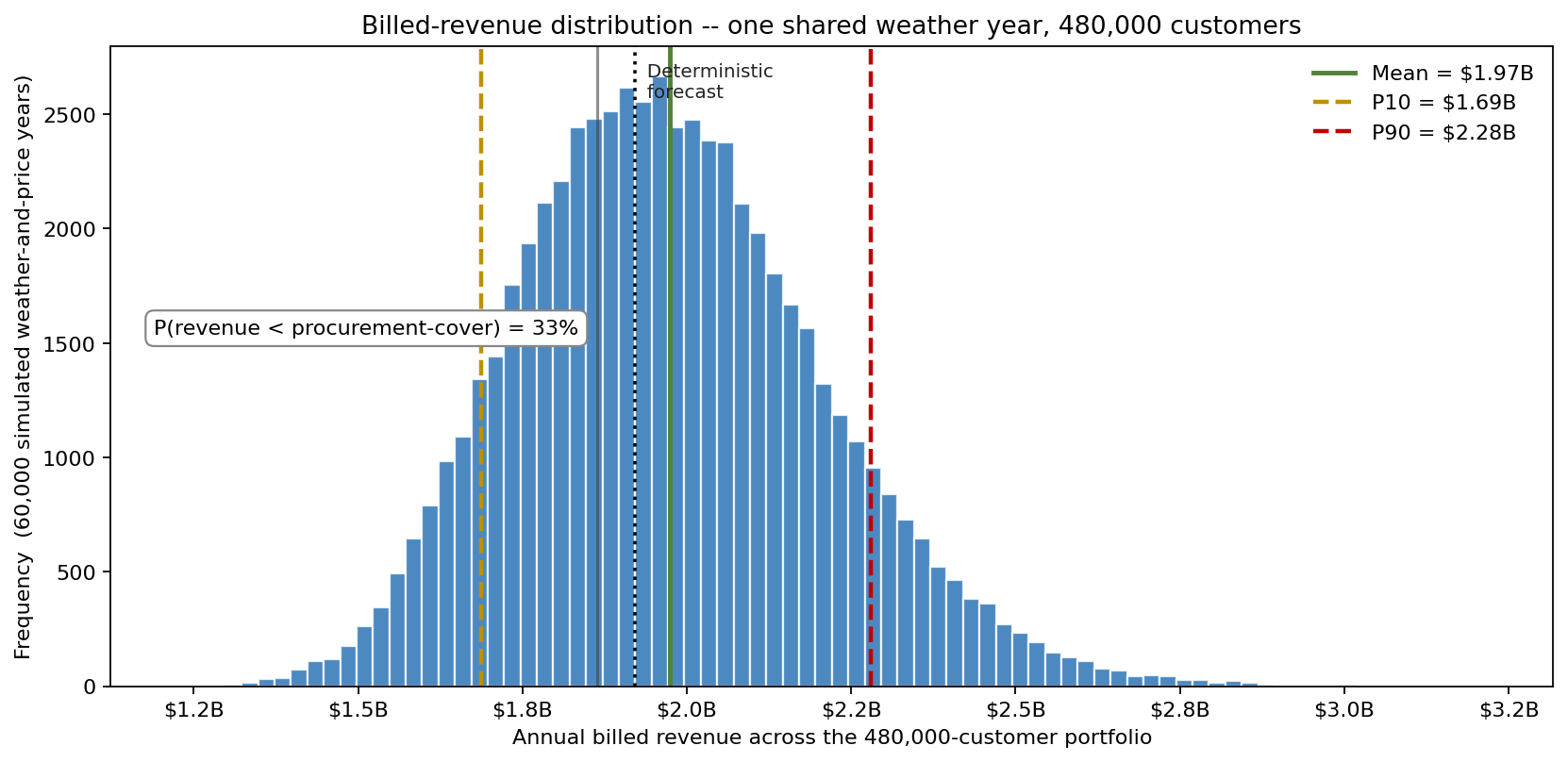
Rebuilt in ModelRisk, the same portfolio produces a mean of $1.97B in billed revenue with a P10 of $1.69B and a P90 of $2.28B — a P10-to-P90 band of $0.59B, fully 30% of the mean. That band is not noise that disappears with scale; it is the footprint of a shared weather year. The chart below is the picture the point estimate could not show.

Why a point estimate fails here

The intuition that a half-million-customer portfolio should be predictable is the classic central-limit trap. It would hold if each customer's consumption were independent — the law of large numbers would crush per-customer variation toward zero. But a hot summer raises the air-conditioning load of every residential customer simultaneously, a cold snap drives every heating load up together, and that common shock does not diversify away. Model the weather year as one standardised anomaly applied to all customers, and the portfolio keeps a 30%-wide revenue band no matter how many meters you add. Freeze that anomaly at its central value — as the deterministic plan silently does — and you forecast the mean while pricing none of the spread.

The deterministic $1.92B sits just below the simulated P50 of $1.96B, because the blended price is right-skewed: fuel pass-through spikes upward more often than it falls. The single number is not wrong so much as blind — it reports the centre and hides the 33% chance that revenue lands below the level needed to cover hedged procurement.

Building the portfolio from one shared weather draw

Each simulated year starts with a standardised weather index W ~ Normal(0,1), fattened with a small Student-t(4) component so genuinely extreme years carry weight. That single draw scales the weather-sensitive share of every customer class — 34% of residential load, 22% of small-commercial, 10% of large-commercial — by roughly +9% per standard deviation. A +1σ year adds about 0.30 TWh of cooling-and-heating load across the book.

Three customer classes carry distinct economics: 86% residential at ~9,200 kWh/yr, 12% small commercial at ~41,000 kWh/yr, and 2% large commercial at ~620,000 kWh/yr. Per-customer behavioural scatter is modelled as a class-level LogNormal, but its coefficient of variation shrinks as 1/√(class size) once pooled — which is precisely why it ends up small relative to the shared weather factor, and why the weather term dominates the spread. Customer-count growth (+1.2% ± 0.6%) and a commercial-activity swing (±1.8%) round out the drivers. Revenue applies a blended tariff drawn LogNormal around $0.158/kWh, with a 30% chance of a mid-year regulator re-rate adding 3–11%.

Three weather regimes, three consumption curves

Conditioning the simulated years on the weather index separates the portfolio into mild, normal, and hot/peaky regimes — the cleanest way to see how much of the uncertainty is weather and how much is everything else.

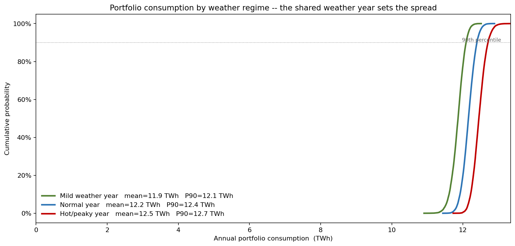
A mild year averages 11.85 TWh, a normal year 12.16 TWh, and a hot/peaky year 12.46 TWh — a 0.6 TWh swing in the central estimate driven by weather alone, before any behavioural or economic uncertainty is layered on. The three CDFs barely overlap, which is the visual signature of a systematic driver: it shifts the whole curve rather than just widening it.

What actually moves the revenue number

The lower tail of revenue — the P10 that procurement hedges against — is what the budget depends on. Ranking the drivers by their effect on P10 billed revenue puts the answer beyond argument.

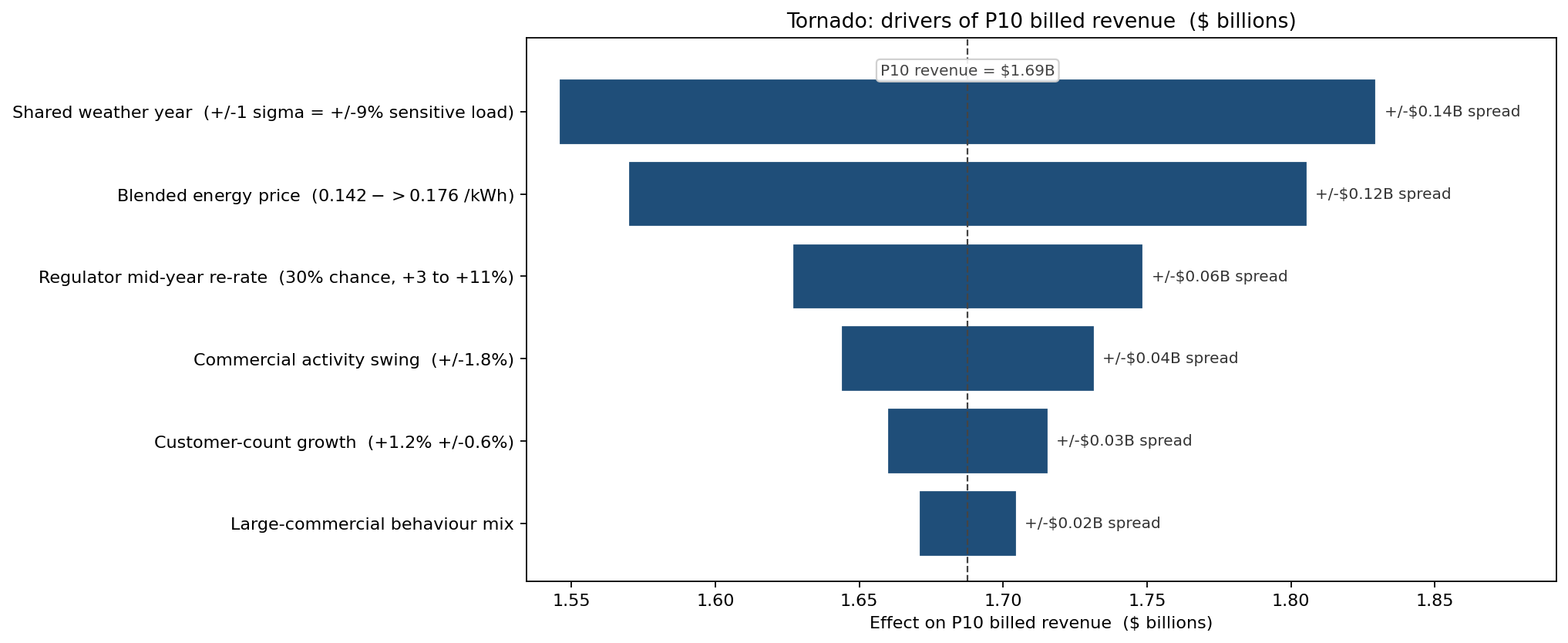
The shared weather year is the largest driver at ±$0.142B of P10 revenue, ahead of the blended energy price (±$0.118B) and the regulator re-rate (±$0.061B). Customer-count growth and class mix — the variables the planning team spent the most effort refining — move the tail by less than ±$0.03B each. The lesson is uncomfortable: the most carefully forecast inputs were not the ones that mattered.

Where the weather risk lives in the year

Annual totals hide when the exposure bites. A monthly fan chart, driven by the same shared weather draw plus a seasonal degree-day shape, shows the risk concentrating where the system is already stressed.

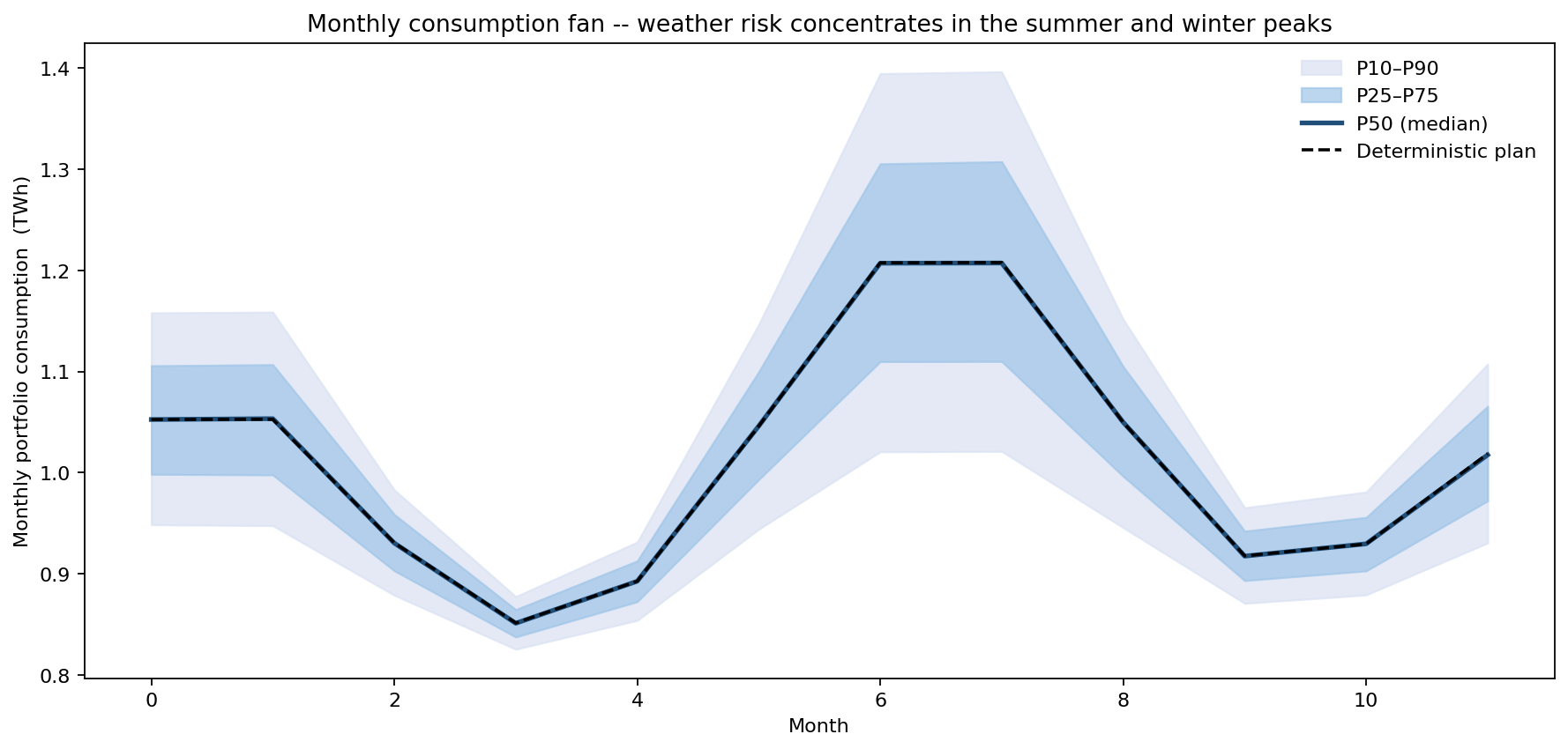
The summer peak month has a median of 1.21 TWh but a P90 of 1.40 TWh — a 15% upside spread concentrated in exactly the weeks when wholesale prices and grid stress are highest. The deterministic plan's flat peak of 1.21 TWh is a coin-flip, not a ceiling.

What the model changed

• Procurement was re-hedged to the P75 of the weather-sensitive load, not the point forecast, after the simulation put the chance of revenue falling below the procurement-cover line at 33% — a one-in-three shortfall the single number rated at zero.
• The summer peak hedge was sized to the P90 month (1.40 TWh) rather than the median, closing the exposure the annual total had averaged into invisibility.
• Forecasting effort was redirected from customer-count refinement (±$0.03B tail effect) to weather-year scenario design (±$0.142B), where an hour of analyst time actually changes the answer.
• The rate-case filing carried the full P10–P90 band, giving the regulator the 30% revenue uncertainty explicitly rather than a false-precision point estimate.

ModelRisk functionality used

• A single shared weather index applied across all 480,000 customers, which is what preserves the 30%-wide revenue band instead of letting it collapse to the mean — the modelling decision the whole analysis turns on.
• LogNormal blended-price draw with a 30%-probability regulator re-rate branch, capturing the right-skew of fuel pass-through that places the deterministic figure below the simulated median.
• Scenario conditioning on the weather index to split the output into mild / normal / hot-year CDFs (11.85 / 12.16 / 12.46 TWh) without re-running the model.
• Tornado on P10 revenue rather than the mean, because procurement hedges the lower tail and the driver ranking there is what sizes the hedge.
• Monthly fan chart seasonalising the shared weather draw to locate the P90 = 1.40 TWh summer peak the annual total concealed.

For a utility, "next year's consumption" is not a number — it is a distribution whose width is set by one weather year shared across every customer, and the only honest budget is the one that prices that width.