Industry: Transportation
Product: ModelRisk
Application: Delivery Scheduling

How Many Drivers Belong in the 4 PM Slot? A Probabilistic Answer

Grocery e-commerce lives on the 2-hour delivery window. The customer picks 4-6 PM Tuesday at checkout; the operator promises a same-window arrival or eats a small refund and a large reputational hit. The headline service-level target is 95% on-time. The deterministic scheduler — orders forecast × average service time ÷ driver minutes — said 12 drivers staffed the Tuesday late-afternoon window comfortably. The chart below tells the story the scheduler could not: at 12 drivers the mean on-time rate is a comfortable 97.4%, but the distribution has a fat left tail — the 10th-percentile day delivers only 89.0%, and the 95% SLA is missed on 17.3% of Tuesdays. The days it misses are not random; they are the days the order count spikes above the forecast mean.

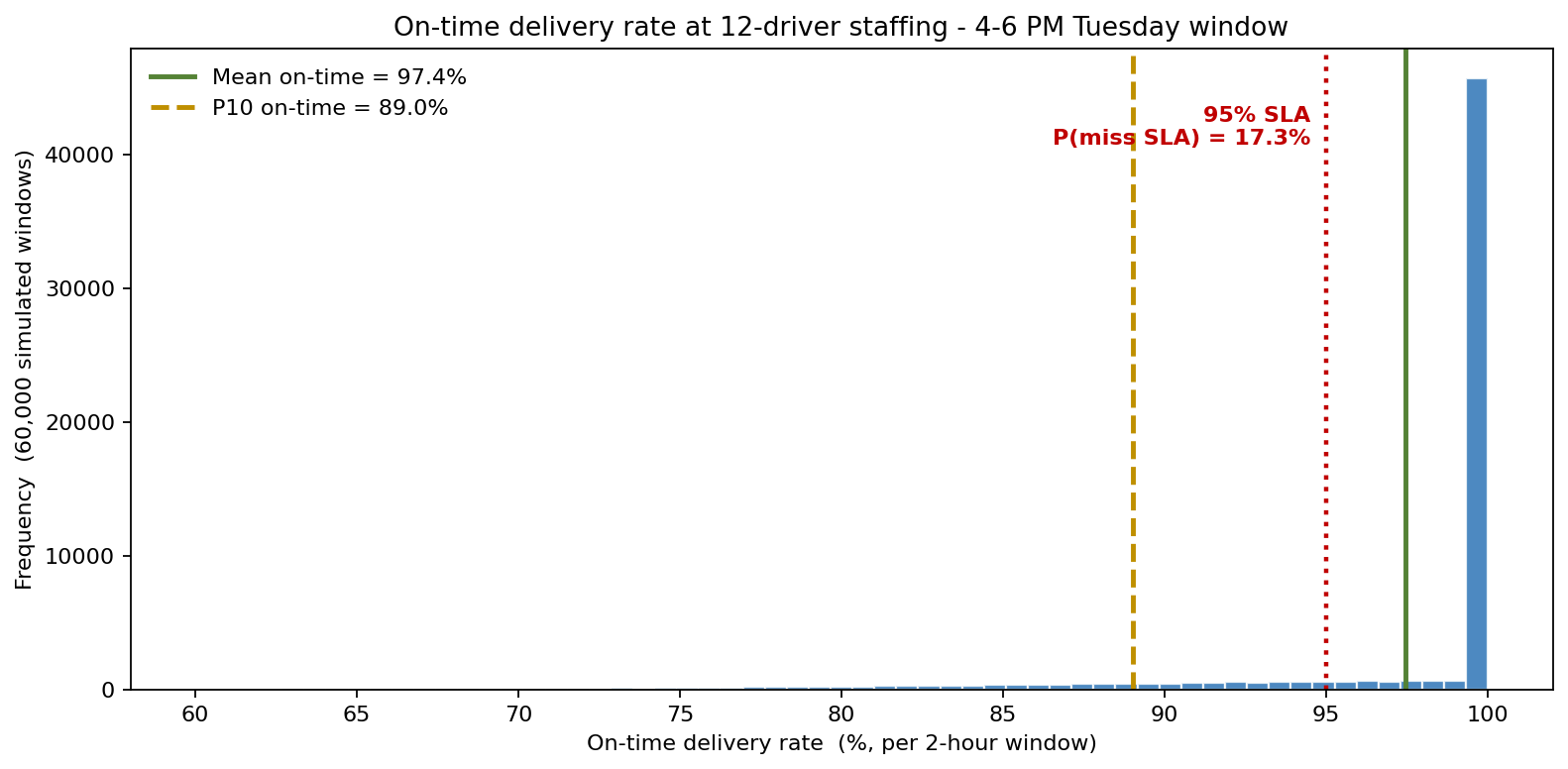
A national grocery chain rebuilt the slot-staffing model in ModelRisk after a quarter of customer-complaint data made clear that the deterministic model was systematically under-staffing during demand surges. The problem was not the wage rate or the service-time assumption — both were close to historical averages. The problem was that the demand distribution had a fatter right tail than a Poisson model assumed, and the deterministic scheduler had no way to see it.

Where the order count actually lives

Eighteen months of order data for the 4-6 PM Tuesday window in the chain's largest metro fulfilment region showed a sample mean of 92 orders and a sample variance of 334 — a variance-to-mean ratio of 3.6. A pure Poisson would have variance equal to the mean. The over-dispersion comes from latent shocks: a school-day shift, a payday cluster, a weather event, a competitor stock-out — none of which the day-of forecast captures.

The right structural choice is a Negative Binomial with mean 92 and dispersion parameter \(r = 35\), which reproduces the observed mean and variance. Using a Poisson here — as the deterministic model implicitly does whenever it "adds a 10% buffer to the mean" — understates the 90th-percentile order count by 12 orders (NegBinomial P90 = 116 vs Poisson P90 = 104). Twelve more orders at 9 minutes apiece is over 100 driver-minutes the schedule did not budget for.

Per-order service time (depot loading → drive → park → handoff → payment) was fitted as LogNormal with mean 9 minutes and CV 0.40 from delivery-app timestamps. The CV-0.40 is what makes a grocery delivery slower-tailed than a parcel toss: occasional payment issues, gated communities, perishable handoff. A driver works the full 120-minute window, but inter-drop transit, the depot loading ramp, and the hard window edges mean only about 78 minutes resolve into completed on-window service — the effective capacity against which order-minutes are charged.

What 12 drivers actually delivers

The deterministic answer — 92 orders × 9 minutes = 828 demand-minutes, vs 12 × 78 = 936 capacity-minutes — said "you're inside capacity, you're fine." The simulation says the mean on-time rate is 97.4% but the 10th-percentile day delivers only 89.0%, and the probability of missing the 95% SLA threshold is 17.3%. The miss is not driven by a generic capacity shortfall; it is driven by tail demand days when the Negative Binomial draws 115+ orders and the per-order service times also run long.

This is the "Why Monte Carlo" beat: the deterministic point estimate sits above the mean, but the SLA is enforced at the window level, not the mean, and 17.3% of windows is a customer-service problem the deterministic answer literally cannot quantify.

Three staffing policies, three cost distributions

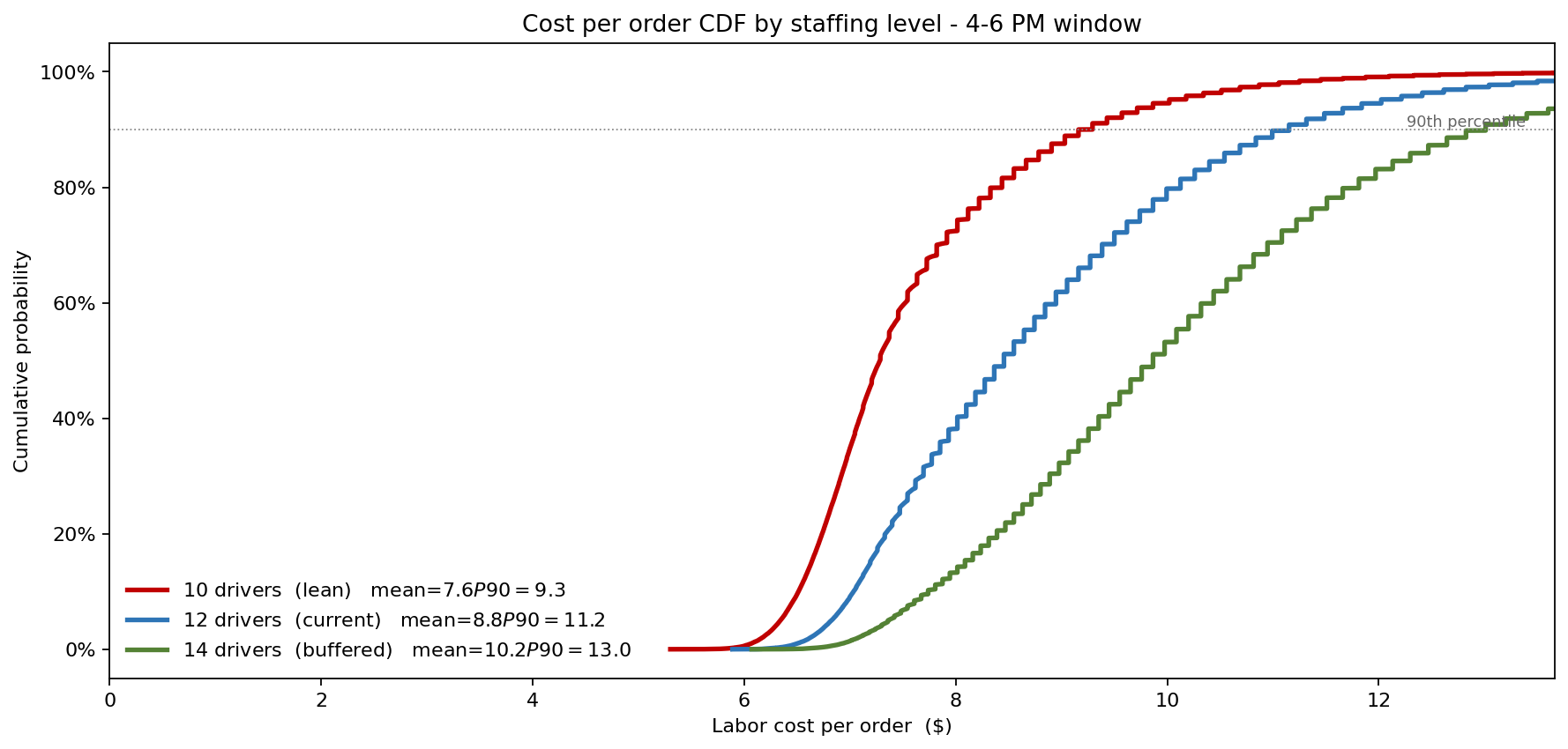
Stripping out the headline number and showing the full distribution makes the staffing trade-off explicit. The lean policy (10 drivers) has the cheapest mean day at $7.63 per order but a long right tail of late-order penalties — and an on-time rate that misses the 95% SLA almost half the time. The current policy (12 drivers) costs $8.82 per order on the mean; the buffered policy (14 drivers) costs $10.19 and all but eliminates late penalties. Cost rises monotonically with crew size — there is no free lunch where adding drivers pays for itself — so the decision is explicitly a price paid for SLA insurance, not a cost minimisation.

The CFO's question shifts. It is no longer "what staffing minimizes mean cost?" but "what staffing meets the 95% SLA on most days at an acceptable cost?" The model's answer for the 4-6 PM Tuesday slot is 13 drivers — at $9.48 per order it cuts the SLA-miss rate from 17.3% to 8.4% and lifts the P10-day on-time from 89.0% to 96.7%. It is a number the deterministic optimizer never proposed, because the deterministic optimizer has no tail to defend against.

What actually moves the cost number

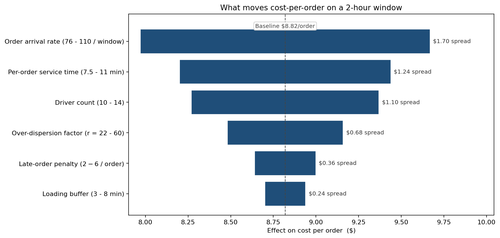
The biggest mover is order arrival rate — the demand draw itself (a $1.70 swing in cost-per-order). Per-order service time ranks second ($1.24), driver count third ($1.10). Critically, the over-dispersion parameter is the fourth-largest mover, worth a $0.68 swing in cost-per-order. This is the parameter the deterministic model assumes away by treating demand as deterministic; that $0.68 of spread translates directly into the value of better demand forecasting upstream.

From insight to action

• Slot staffing now optimized window-by-window. Each of the 14 standard delivery windows has its own NegBinomial demand fit and its own optimal staffing curve. The Saturday morning window — historically thought to need the same crew as Tuesday afternoon — turned out to need 17 drivers because its dispersion parameter is half that of the weekday windows.
• Slot-yield management retuned. Demand-day forecasts that trigger an upper-tail flag (predicted demand > P85 of the NegBinomial) now auto-recommend cap-and-divert: the booking engine closes the slot earlier and offers free 30-minute window flexibility to redistribute orders to the adjacent slot.
• The "95% on 95% of days" SLA contract replaced the "95% on average" contract internally. The simulation gave operations the language to defend a 30 cents-per-order incremental labor budget that earlier had been treated as overspending.

ModelRisk Functionality Used

• Negative Binomial demand fitting to the 18-month order-count history per window, with the over-dispersion parameter \(r\) fit by maximum likelihood — exposing the 3.6 variance-to-mean ratio the Poisson-style planner had hidden.
• LogNormal service-time fitting (mean 9 minutes, CV 0.40) from delivery-app timestamps, with the fit dialog used to confirm that a Normal fit produced a 7% probability of negative service times — disqualifying it on first principles.
• 60,000-iteration window simulation that produced both the on-time-rate distribution and the cost-per-order distribution, side-by-side, at each candidate staffing level.
• Scenario comparison across 10, 12, and 14 driver staffings on identical demand draws — making the CDF comparison apples-to-apples and the policy decision defensible against the "but my staff cost more under the buffered plan" objection.
• Tornado ranking of the six cost drivers — surfacing the over-dispersion parameter as a top-five mover and turning it into a business case for an upstream demand-forecasting upgrade.
• Threshold probability outputs in the format the customer-experience team needed: P(window on-time < 95%) per slot per day-of-week, plugging directly into the SLA-monitoring dashboard.

A delivery window is not an average; it is a probability that a particular evening's order draw will fit inside a particular evening's driver capacity. Monte Carlo simulation in ModelRisk turns the staffing question from "what's the expected utilization?" into "what staffing keeps tail-day SLAs intact?" — and that reframing is what moves the operations committee.