Industry: Telecommunications and IT
Product: ModelRisk
Application: Software Scalability

Auto-scaling a streaming microservice when viral spikes are part of the traffic shape

A consumer-streaming microservice carries roughly 12,000 requests per second on average, with a diurnal swing between 3,600 rps overnight and 20,000 rps at the 8 p.m. peak. Once or twice a week — call it 0.8% of busy minutes — a content drop, a creator going viral or a push-notification campaign multiplies the steady-state load by a Pareto factor whose median is about 5× but whose power-law tail reaches well past 100× for a few minutes. The deterministic capacity plan, sized at the 95th-percentile diurnal load, picks a static fleet of 20 instances and reports the SLO is met. The Monte Carlo simulation — sampling diurnal, lognormal noise and viral-spike multipliers per minute and feeding the result through a Universal Scalability Law model of per-instance throughput — reports the static fleet blows the 350 ms P99 SLO in 8.5% of minutes, with a P99 latency near 1 second. A predictive auto-scaler trained on a 5-minute-ahead forecast cuts that to 3.4%, for an annual cost bill that is actually lower than the static fleet's.

The four policies fan out across the latency distribution below: the static fleet and the lagging reactive policies straddle or blow the SLO, while the predictive policy pulls the bulk of the distribution inside it.

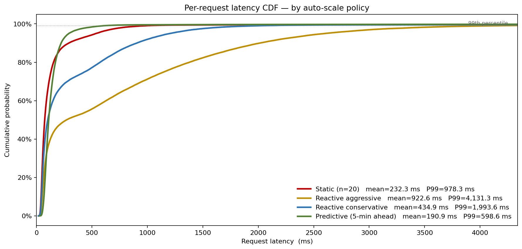
That comparison — static loses on quality and cost — is exactly the kind of conclusion a point-estimate sizing exercise cannot produce.

The arrival shape has three components

Per-minute arrival rate was modeled as the product of three independent factors:

• Diurnal envelope. A sinusoidal shape between 0.30× and 1.70× the steady-state rate, peaking at 8 p.m. local. This is the predictable component a scheduling policy can pre-warm against.
• Lognormal multiplicative noise with σ = 0.20, capturing the minute-to-minute variability that even a stable user base produces.
• Viral-spike Pareto multiplier. A Bernoulli(0.008) flag fires a Pareto(α = 1.4) multiplier on top of the baseline arrival; the heavy tail means a typical spike is a ~5× excursion, but the 99th percentile of spike size runs past 150× — and it is precisely that tail that no fixed fleet can absorb.

Pareto, not LogNormal, is the right distribution for the spike multiplier because the tail of viral-content propagation is power-law on every dataset that has been published. Substituting LogNormal here would clip exactly the tail that drives the SLO breaches.

Per-instance throughput is not linear in fleet size

The second mistake the deterministic plan made was assuming horizontal scaling is linear: 20 instances at a nominal 2,000 rps each = 40,000 rps of capacity. In practice every microservice runs into Universal Scalability Law (USL) behaviour as the fleet grows:

capacity(n) = n × μ / (1 + α(n − 1) + β·n·(n − 1))

The α term captures serialised work (config refresh, leader election, shared cache lookups); the β term captures inter-node coherency cost (cross-AZ chatter, distributed-lock contention). For the platform's measured profile (α = 0.03, β = 8e-5), a fleet of 20 instances actually delivers about 25,000 rps of useful capacity, not 40,000 — a 38% effective haircut at the headline scale. The model uses USL throughput at every fleet size, not the linear-extrapolation cartoon.

Four auto-scale policies

Four policies were simulated against the same 60,000-minute synthetic traffic trace:

• Static fleet (n = 20). No scaling. Cheap to operate, no scheduler complexity — and at a P99 latency near 1 second it blows the SLO 8.5% of minutes, whenever a viral spike fires on a fleet that cannot grow.
• Reactive aggressive. Scales to maintain 70% utilisation at +10% headroom, with a 2-minute observation lag and 30%-per-decision step. The lag is fatal: P99 climbs past 4 seconds and it breaches 48% of minutes.
• Reactive conservative. Targets 55% utilisation at +30% headroom, 3-minute lag, 15% step. The "safe" choice still breaches 28% of minutes (P99 ≈ 2 s).
• Predictive (5-minute ahead). Uses a forecast of the next 5 minutes' arrival to pre-warm the fleet before the spike hits. Effectively zero lag, 40% step, 20% headroom — P99 ≈ 600 ms, breaching just 3.4% of minutes.

What the deterministic-sized plan missed

The static fleet sits at a P99 latency near 1 second, and the lagging reactive policies are far worse — the queueing-and-overflow formula returns multi-second results once a viral spike pushes ρ over 1.0 on a fleet that is either fixed or chasing the spike too late. The predictive policy pulls almost the entire distribution inside the SLO; the residual 3.4% of breaching minutes are the most extreme power-law spikes that no fleet of ≤120 instances could serve.

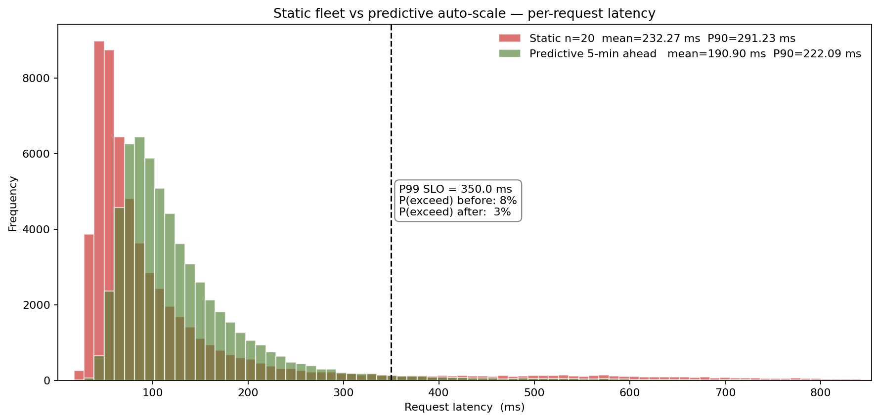
The before/after framing is the conversation the engineering manager actually has to have with the CFO: "for less money, we pick the policy whose latency distribution sits inside the SLO instead of straddling it."

What actually moves the P99

Sensitivity ranking under the predictive policy tells the team where to invest in modeling effort versus engineering effort.

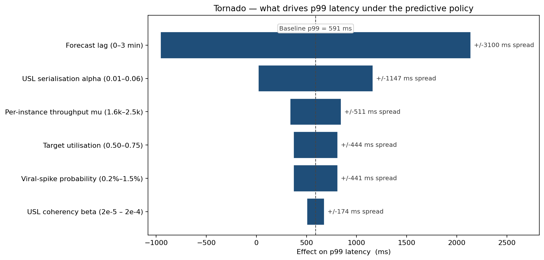
The dominant lever is forecast lag — moving from a zero-lag pre-warm to a 3-minute-stale forecast swings P99 latency by more than 3 seconds. That single result is what justifies the data-engineering investment in the 5-minute-ahead model: the entire value of the predictive policy lives in acting before the spike, not after. USL serialisation α is second, and unlike the spike itself this is something the platform team controls directly via cache architecture and lock granularity. Per-instance throughput and target utilisation come next; viral-spike probability and coherency β move P99 the least once the forecast is in place — a useful robustness result, since the spike rate is the variable the team has no control over.

The cost-quality scatter the procurement team sees

Annual cost combines compute (instance-minutes × cloud rate) and SLA-credit exposure (priced at $20,000 per percentage-point of breached minutes per year). Plotting each policy as a single (breach %, $M/yr) point makes the dominated options obvious.

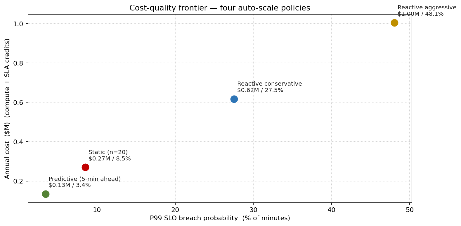
The reactive policies sit in the worst corner — the aggressive one is the single most expensive option at $1.0M/yr, almost all of it SLA credit, because its 2-minute lag means it is perpetually a step behind the spikes. The static fleet is middling at $0.27M/yr ($0.10M compute always provisioned for peak, $0.17M SLA). The predictive policy is Pareto-dominant at $0.13M/yr: lower compute cost (because it deprovisions during the long overnight valley) and lower SLA cost (because it scales ahead of spikes). The annualised gap between the static plan and the predictive policy is roughly $0.14M — and against the reactive-aggressive trap the predictive policy saves nearly $0.9M/yr. None of it is visible to a deterministic capacity plan that sized to the diurnal peak and called it done.

What changed

• Predictive auto-scaler funded and deployed, sized off the simulated P99 latency rather than the deterministic 95th-percentile load.
• 5-minute-ahead arrival forecast added to the platform observability stack, because the tornado showed forecast lag was the single largest P99 mover — and the cheapest to fix.
• Lock-granularity refactor on the catalog service prioritised after USL α was ranked second in the tornado — the engineering investment with the next-highest P99 leverage.
• Static-fleet plan retired for this microservice and the same model exported as a template for the other 14 services on the same architecture.

ModelRisk functionality used

• Three-factor arrival model (diurnal × LogNormal noise × Pareto viral multiplier), composed inside ModelRisk with VoseLognormal2 and VosePareto, so the viral tail is priced in the same simulation as the diurnal envelope.
• Universal Scalability Law per-instance throughput, written as a single Excel formula on the fleet count, so the simulation never assumes linear horizontal scaling.
• Auto-scale policy comparison via overlaid latency CDFs, letting the team read SLO compliance off one chart rather than four.
• Sensitivity ranking on P99 latency, which separated the variables the platform team controls (USL α, forecast lag) from those it does not (viral-spike probability) — directing engineering effort to where it pays off.
• Cost-quality scatter of (breach %, $M/yr) for each policy, making the Pareto-dominant choice visually obvious to the CFO.

Software scalability is not the number of instances at peak; it is the joint distribution of arrival rate, USL-degraded capacity and scale-controller lag — and the SLO is a quantile of the latency distribution that depends on all three. Monte Carlo simulation in ModelRisk is what turns "the static fleet meets the SLO at 95th percentile load" into "the predictive policy holds the SLO breach rate to 3.4% across the full distribution of viral-spike futures — versus 8.5% for the static fleet — for less money than the static plan."