Industry: Retail
Product: ModelRisk
Application: Demand Forecasting

The mean forecast says order 5,000 jackets; the newsvendor math says 6,196

A buyer had one decision to make for the coming season: how many units of a single fashion jacket to commit to, before a single one had sold. The planning system did what planning systems do — it averaged the history, applied a seasonal index, and printed a point forecast of 5,000 units. The buy was set to match. Order the forecast, the logic went, and you can't be far wrong.

The Monte Carlo rebuild in ModelRisk said the point forecast was almost the worst number to order. Once season demand is treated as a distribution rather than a single figure — mean 4,990 units but with a standard deviation of 2,039 units, a P10 of 2,618 and a P90 of 7,699 — and once the economics of getting it wrong are made explicit, the profit-maximising order rises to 6,196 units, almost a quarter above the forecast. Ordering the mean leaves an estimated $8,091 of season profit on the table and runs a 44% chance of stocking out.

Why a single demand number fails here

Two things break the point forecast. First, season demand for one SKU is not a tidy bell. A shared seasonal/macro factor — a warm winter, a soft consumer mood — scales the whole season up or down at once, so the demand distribution is over-dispersed and right-skewed (variance far above the mean, unlike a thin Poisson). The mean sits well to the left of the long upside tail. Second, the cost of being wrong is asymmetric. Each unsold jacket is marked down from a $40 landed cost to a $22 salvage value — a $18 loss. Each unit short is a lost sale of the $55 margin. Understocking hurts three times as much as overstocking, so the right order is not the mean — it is the demand quantile where those two costs balance. That balance point, the newsvendor critical fractile, is $55 / ($55 + $18) = 75%. The buyer should plan to stock out only one season in four, not one in two.

Season demand for one SKU is over-dispersed, not a tidy bell

The whole decision starts with the shape of demand:

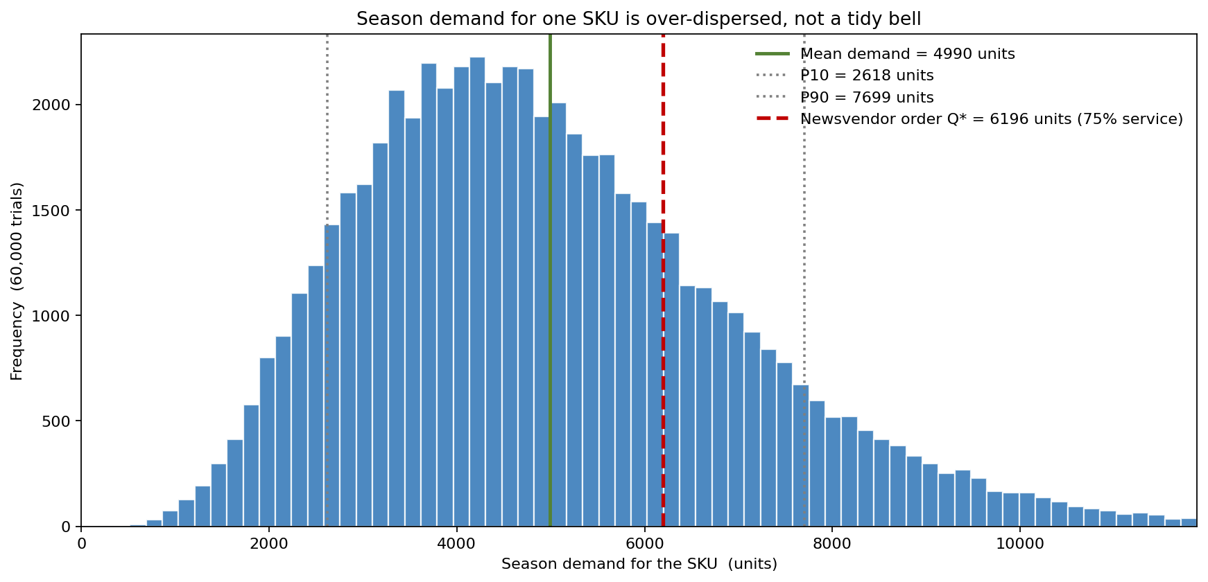
Demand has a mean of 4,990 units and a standard deviation of 2,039 — a coefficient of variation of 0.41, far wider than the Poisson a naive count model would assume. The P10 is 2,618 and the P90 is 7,699, a spread of more than 5,000 units around a 5,000-unit forecast. The distribution is visibly right-skewed: the median (4,714) sits below the mean, and a long upside tail of strong-season outcomes pulls the average up. The naive mean order of 5,000 units sits near the middle of the body, while the newsvendor order of 6,196 units — the 75th percentile — sits out on the right shoulder, deliberately covering most of the upside. A model that reports only "5,000" cannot tell the buyer that the right place to stand is the 75th percentile, not the 50th.

Where the profit actually peaks: the service-level sweep

Sweeping the order quantity from a 50% service level up to 99% shows expected profit rising, peaking, then falling as overstock losses take over:

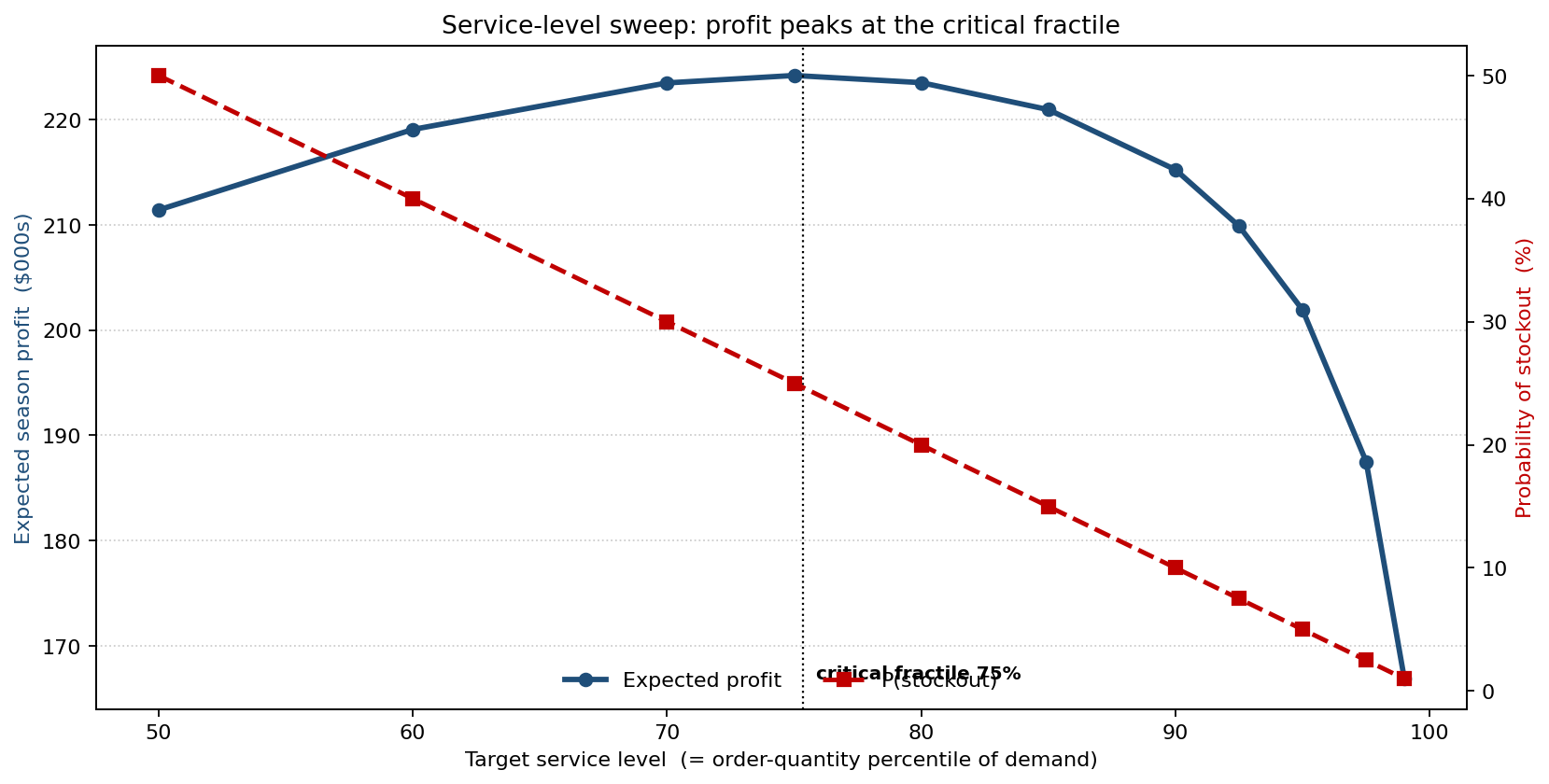
Expected season profit climbs from $211,408 at a 50% service level (order 4,714), peaks at $224,186 at the 75% critical fractile (order 6,172), and then declines — at a 95% service level (order 8,749) profit has fallen back to $201,904, and at 99% (order 10,915) to $166,880, eaten alive by markdowns on unsold stock. The probability of stockout falls monotonically from 50% to 1% along the same axis, which is exactly why "just don't stock out" is the wrong objective: chasing a 99% service level destroys profit. The peak is flat-topped near the optimum, but it is unambiguously not at the mean order: the naive 5,000-unit buy returns $216,098 and stocks out 44% of the time, while the 6,196-unit newsvendor order returns $224,189 — $8,091 (3.7%) more — and stocks out 25% of the time.

The understock / overstock trade-off, made explicit

The same optimum can be read as the point where two opposing costs balance:

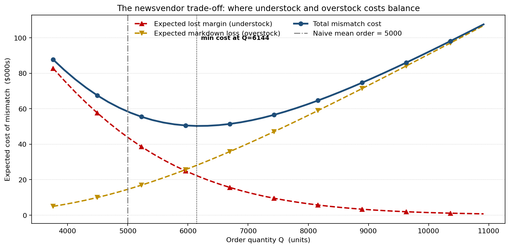
The expected lost margin (understock cost) falls as the order grows; the expected markdown loss (overstock cost) rises. Their sum — the total cost of mismatch — is minimised at 6,144 units, essentially the newsvendor optimum. At the naive mean order of 5,000, expected lost margin is $43,830 and markdown loss only $14,524, for a total mismatch cost of $58,353 — the model is badly under-ordering, bleeding margin on stockouts. At the 6,196-unit optimum, lost margin falls to $21,514 while markdown rises to $28,748, for a total of $50,263 — about $8,090 cheaper. The crossing of the two cost arms is the visual signature of the critical fractile: the right buy is where the next unit's expected markdown risk just equals its expected lost-margin saving.

What swings the answer

A tornado over the demand inputs shows where the forecast's uncertainty comes from:

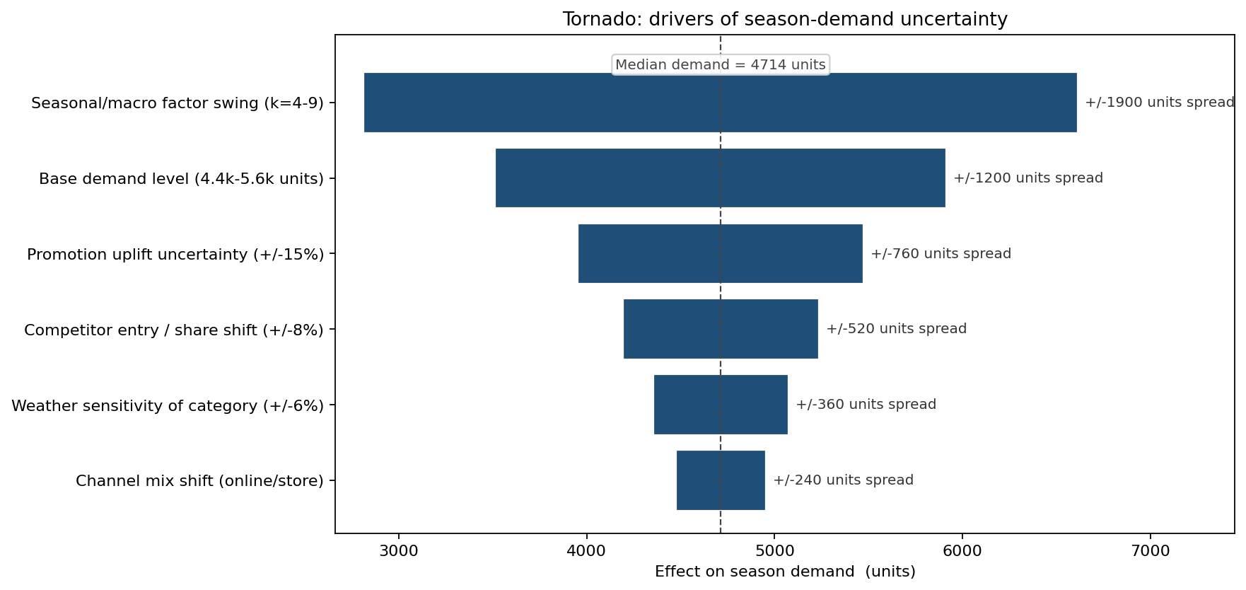
The shared seasonal/macro factor dominates, with a ±950-unit half-spread on season demand — the warmth of the winter and the strength of the consumer matter more than anything the buyer controls. The base demand level is second at ±600 units, then promotion-uplift uncertainty at ±380 and competitor entry at ±260; weather sensitivity (±180) and channel mix (±120) are minor. The ranking tells the planner that tightening the demand forecast means investing in the read on the season itself, not in shaving the smaller operational inputs — and that no amount of forecasting will collapse the spread to a point, which is precisely why the buy should be sized off the distribution.

What the model changed

• The season buy moved from the deterministic 5,000-unit mean forecast to the 6,196-unit newsvendor optimum — a 24% larger commitment that captures an estimated $8,091 of additional season profit on the SKU.
• The planning target switched from "match the forecast" (a 50/50 stockout) to "stock to the 75% critical fractile", an explicit, defensible service level derived from the $55 margin and $18 markdown.
• Stockout probability became a planned quantity, not an accident: 25% by design at the optimum, instead of the 44% the mean order delivered by default.
• Forecasting effort was redirected to reading the season, after the tornado showed the shared seasonal/macro factor — not the controllable operational inputs — is the dominant source of demand uncertainty.

ModelRisk Functionality Used

• Negative-Binomial-shaped season demand built from a shared Gamma seasonal factor over conditional Poisson weekly arrivals, so demand is genuinely over-dispersed (CV 0.41) rather than the thin Poisson a count model would impose — and never collapses to a central-limit bell.
• Critical-fractile newsvendor optimisation computing the 75% service level from the $55 lost-margin and $18 markdown costs, and reading the optimal order straight off the demand distribution at 6,196 units.
• Decision-variable sweep across eleven service levels with a full profit and stockout-probability calculation at each, plotted to locate the profit peak and show that chasing a 99% service level cuts profit by a quarter.
• Cost-decomposition curve separating expected lost-margin from expected markdown loss across the order grid, locating the total-mismatch minimum at 6,144 units.
• One-at-a-time tornado ranking the seasonal/macro factor, base level, promotion uplift, and competitor entry by their effect on season demand, directing forecasting effort to the season read.

Demand forecasting for a one-shot seasonal buy is not "what is the most likely number of units" — it is "given the shape of demand and the asymmetric cost of being wrong, what quantile should I stock to." The point forecast answered the first question and got the second one badly wrong; ModelRisk answered the one that actually sets the order.