Industry: Real Estate
Product: ModelRisk
Application: Housing Market Analysis

A balanced market and a 5% correction can be the same year — the question is how likely

A deterministic supply-demand model for a single metro plugged in mean inputs and printed a tidy answer: a clearing price index of 101 (essentially flat versus today) and 5.7 months of inventory — a balanced market, nothing to see. The probabilistic re-run, built in ModelRisk over 120,000 draws of the same market, told a sharper story: a 23% chance the price clears more than 5% below today's level, an 8% chance of a correction deeper than 10%, and a 45% chance the market tips into oversupply (more than six months of inventory). The point estimate landed in the middle of a distribution it could not see — and the middle is not where the risk lives.

Why a point estimate fails here

A metro housing market clears where demand meets supply, and both sides are uncertain at the same time for the same reason. When money tightens, mortgage rates rise, qualified-buyer formation falls, and affordability erodes — three blows that land together, not independently. A deterministic model plugs in the central rate, the central formation number, the central completions number, and reads off one clearing price. It cannot represent the scenario that actually frightens an investor: the joint bad draw, where weak demand and a wave of completions arrive in the same year and the price gaps down.

Worse, the clearing-price function is non-linear in the demand-to-supply ratio. Evaluating it at the mean inputs is not the same as the mean of the function — so even the central number a deterministic model reports is biased. Only a simulation that draws demand and supply together, through a shared macro factor, recovers the true shape.

Modeling the market as a supply-demand equilibrium

The model is a snapshot of one metro over one transaction year. A single standard-normal macro/rate factor Z drives the correlated machinery:

• Mortgage rate — centered at 6.5%, loaded on Z so a tight-money draw lifts rates, clipped to a 3%–11% plausible band.
• Demand (qualified buyers, thousands of households) — household formation around 52k, reduced when Z is high, multiplied by an affordability term that decays as the mortgage rate climbs. Formation and affordability load on the same Z, so a recession hits demand on both channels at once.
• Supply (thousands of units) — new completions as a Triangular(18, 24, 31), locked in from permits 18–24 months ago and only loosely tied to today's macro, plus existing-stock listings that drift up modestly with Z.

The market clears through a constant-elasticity inverse-demand relation, price_index = 100 × (demand / supply)^(1/3.2), and months of inventory build from a balanced six-month buffer plus the excess of annual supply over the monthly sales pace. Prices stay positive by construction.

The shared factor is the point of the model, so it was verified directly:

• corr(demand, mortgage rate) = −0.95
• corr(formation, affordability) = +0.86
• corr(clearing price, months of inventory) = −0.97

Demand and rates move strongly opposite; the two demand channels move together; and — the headline relationship — price and inventory are almost perfectly inverse. That last correlation is what makes "oversupply" and "price correction" two faces of one event rather than two independent risks.

Where the market clears, and what it costs

The headline chart is the equilibrium itself — every simulated year as a point in price-versus-inventory space.

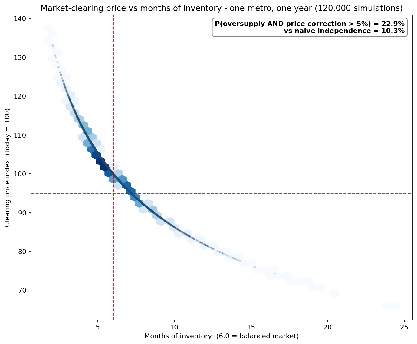
The cloud is a tight downward curve: high inventory and a price correction are the same draws. The vertical line marks the balanced six-month inventory level; the horizontal line marks a 5% correction (index 95). The joint tail — oversupply and a correction deeper than 5% — has probability 22.9%. A naive calculation that treated the two risks as independent would multiply 45% by 23% and report 10.3%, understating the joint danger by more than half. Because price and inventory are nearly co-determined, almost every correction is an oversupply event; the risks are not separable.

How deep could the correction go?

Collapsing the equilibrium onto the price axis gives the cumulative distribution of where the market clears.

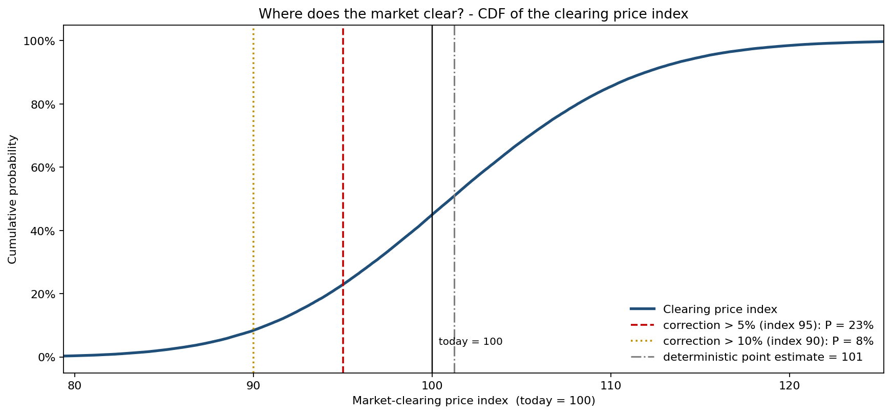
The clearing index runs P10 = 91, P50 = 101, P90 = 112. The deterministic point estimate (index 101) sits right at the median, which is exactly why it is misleading — it reports the center and stays silent about the tail. Read off the thresholds: P(correction > 5%) = 23% at index 95, and P(correction > 10%) = 8% at index 90. The downside is fatter than the upside is thin, the signature of a rate-sensitive demand side.

At what rate does the market tip?

Because the macro factor is the engine, the most actionable question is how the tipping probabilities move as the central mortgage rate is swept.

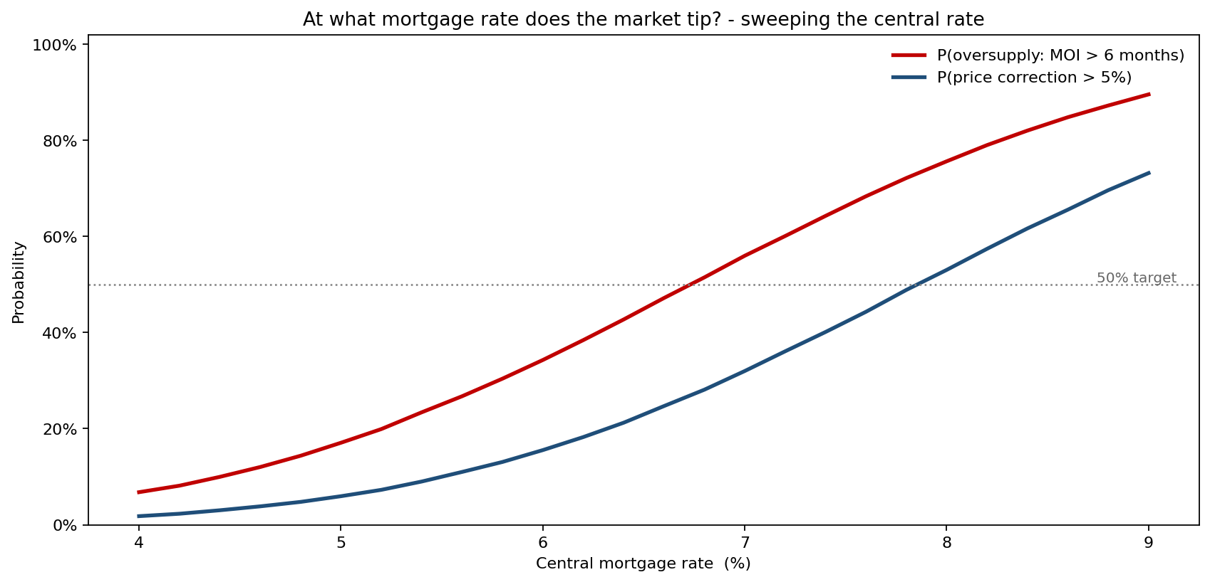
The two curves rise steeply through the 6%–8% band. At a 6% central rate the market faces a 34% chance of oversupply and a 16% chance of a 5% correction; at 7% those become 56% and 32%; at 8% they reach 76% and 53%. The 50% line — the point at which a correction is more likely than not — is crossed near an 8% mortgage rate. That single number reframes the rate-watching: the market does not degrade linearly, it tips.

What drives the spread

Ranking the inputs by their contribution to the clearing-price spread confirms where the uncertainty originates.

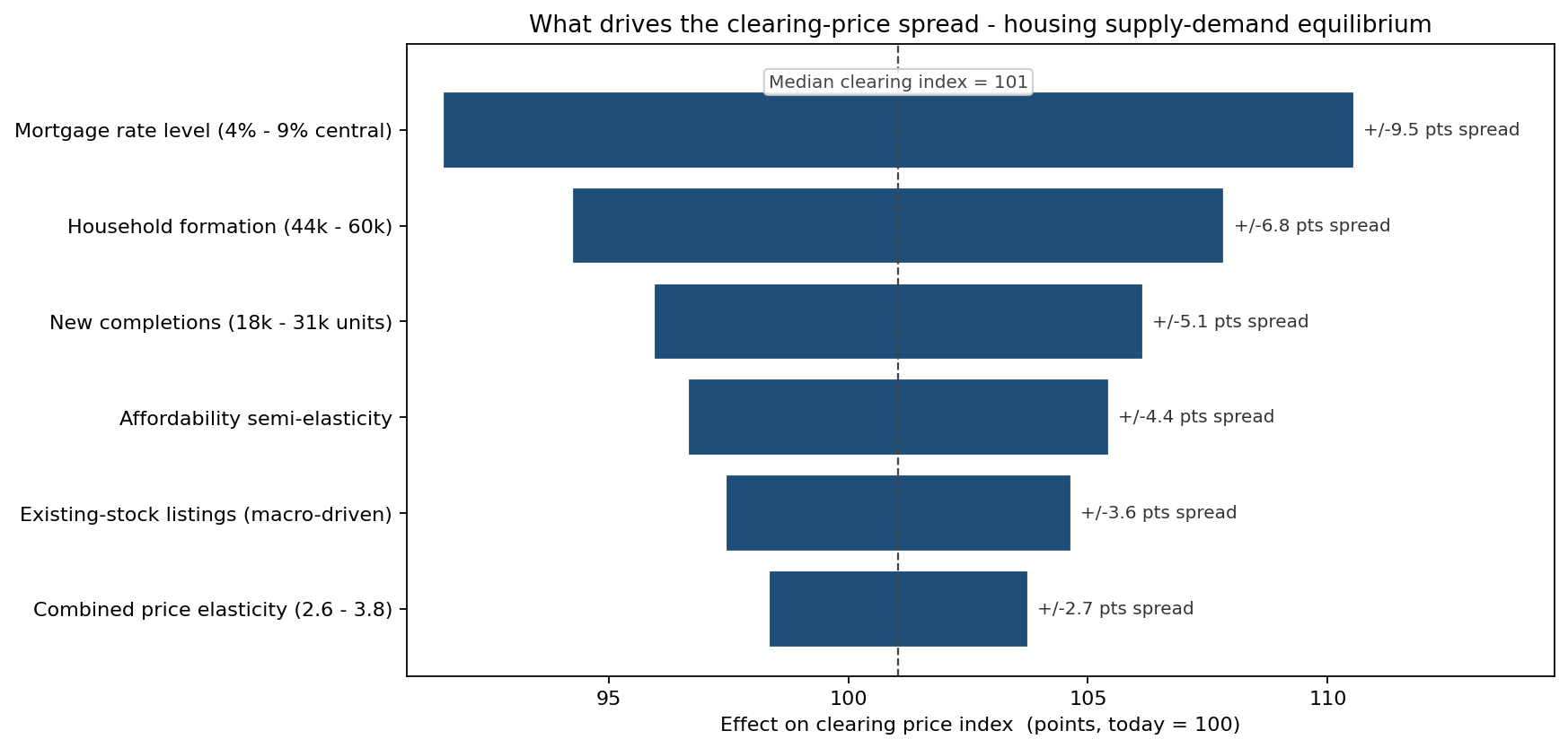
The mortgage-rate level dominates, with household formation and new completions behind it — the demand-side macro channel outweighs the supply-side construction channel, but not overwhelmingly. The takeaway is that monitoring should concentrate on the rate path and formation data, while completions (already largely locked in by permit pipelines) are the more knowable side of the ledger.

What the model changed

The deterministic verdict was "balanced market, hold." The probabilistic verdict was "balanced on average, with a one-in-four chance of a real correction and a one-in-two chance of tipping into oversupply if rates push toward 8%." The firm used the distribution three ways: it sized acquisition contingencies to the P10 clearing price (91) rather than the central case; it set a rate trigger at the 8% tip point for pausing new bids in this metro; and it stopped treating oversupply risk and price risk as separate line items once the −0.97 correlation showed they were one event.

ModelRisk functionality used

• Monte Carlo simulation — 120,000 joint draws of demand, supply, and rates to recover the clearing-price and inventory distributions.
• Common-factor correlation modeling — a single macro/rate factor driving mortgage rates, household formation, and affordability together, verified at −0.95 / +0.86 / −0.97.
• Joint-tail probability outputs — P(oversupply AND correction) reported against the naive-independence product to quantify the dependence.
• Parameter sweep — tipping probabilities traced across the 4%–9% mortgage-rate range to locate the 8% tip point.
• Tornado sensitivity — clearing-price spread decomposed across six structural inputs.

Monte Carlo turns a supply-demand model from a single clearing price into the distribution of clearing prices — the only frame in which "balanced market" and "5% correction" can be recognized as the same year seen at different odds.