Industry: Project Management
Product: ModelRisk
Application: Risk Mitigation

When Three Risks Account for 56% of the Exposure: Quantitative Risk Mitigation

The PMBOK risk register on a $420M LNG-jetty construction project had 47 logged threats. The deterministic Expected Monetary Value (EMV) total was $10.9M — already a number large enough to demand a contingency conversation. But a single number tells the project nothing about the shape of the risk it is carrying. The same register, run through Monte Carlo simulation, returns a right-skewed exposure distribution: most programmes land near the median, a long tail does not, and the contingency the board actually needs sits well above the mean.

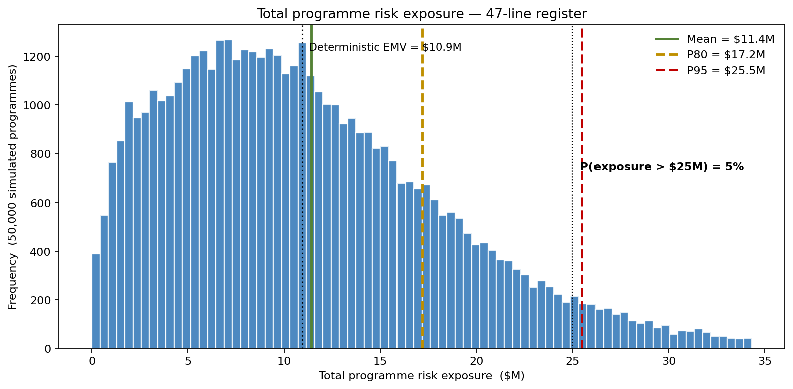
The mean of the simulated exposure is $11.4M — close to the EMV, as it should be — but the P80 is $17.2M (1.6× the EMV) and the P95 is $25.5M (2.3× the EMV). A flat 10% contingency on the deterministic EMV would have been wrong twice over: the wrong percentile, and applied evenly across risks where the mitigation dollars should have been heavily concentrated. The owner used ModelRisk to convert the register from a bookkeeping artefact into a prioritized mitigation budget.

Modeling the register

Each line in the risk register has three uncertain things: the probability the risk fires, the cost impact if it does, and the duration impact (often correlated with cost). Treating these as point estimates and multiplying them — the classic EMV calculation — collapses the distribution to a single number and discards the information the project actually needs.

Risk probability. Modeled as Beta, parameterised so that low-frequency risks (Beta(2, 18), mean ≈ 0.10) and credible-but-not-likely risks (Beta(5, 10), mean ≈ 0.33) had appropriately skewed shapes rather than the symmetric error bars a Normal would impose.

Cost impact (given the risk fires). LogNormal for cost-overrun events with long right tails — e.g. monsoon-driven re-work, LogNormal(μ = log(3.6), σ = 0.55), mean ≈ $4.2M, P90 ≈ $7.3M. The lognormal mean uses exp(μ + σ²/2), not exp(μ); using the median in place of the mean is a 15–25% systematic under-estimate for these shapes.

Duration impact. PERT with a tight floor and a long ceiling — e.g. permit-delay PERT(10, 30, 95) days.

Correlated firing (shared root cause). Lines that share a root cause do not fire independently. The monsoon, foundation-soils, and marine-spread lines all load on a shared weather-window factor (Gaussian-copula factor loading 0.6), and the permit and stakeholder-hearing lines share a regulatory-cycle factor (loading 0.5) — so they genuinely co-fire in the same iterations. The empirical pairwise firing correlation that results is ≈ 0.22 within the weather group and ≈ 0.14 within the regulatory group, while unrelated lines stay near zero. This is what fattens the right tail: in a bad year, the correlated risks land together.

Three of the 47 register lines came in heavy on this re-pricing — monsoon-window slip, foundation-soils discovery, and an upstream-supplier customs hold — and together they drove most of the tail.

What deterministic EMV hid

The deterministic register added probability × cost to $10.9M EMV — a single point on a wide distribution. The simulated mean is close to that EMV (it should be — the mean is the sum of the per-line expected values), but the P80 is 1.6× the EMV and the P95 is 2.3×, because the correlated tail carries the programme well past the average. A 10% contingency on the EMV figure of $10.9M ($1.1M) was nowhere near enough; the appropriate contingency for an 80% confidence target was about $5.8M above the mean (P80 minus mean), and concentrating that money on the right risks mattered more than the size of the pot.

Where the exposure lives — the Pareto

A Pareto over the 12 largest contributors revealed the concentration the deterministic register did not surface.

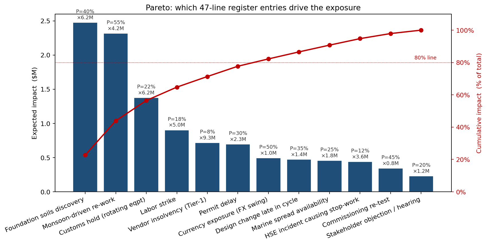
Three lines — foundation soils, monsoon re-work, and the customs hold on rotating equipment — accounted for 56% of the expected impact and an even larger share of the tail variance. Mitigation budget should chase that 56%, not the long tail of 1–3% lines that absorbed equal management attention before the analysis.

Mitigation evaluated, not advocated

Two mitigations were compared by re-running the same simulation against the modified register, not against gut feel:

1. Pre-season monsoon shelter package ($1.8M capex). Reduces the cost-impact distribution on monsoon re-work from LogNormal(μ = log(3.6), σ = 0.55) to LogNormal(μ = log(1.4), σ = 0.40), and reduces the firing probability from 0.55 to 0.30.

2. Diversified supplier with parallel customs clearance ($0.9M setup). Reduces the customs-hold firing probability from 0.22 to 0.07, and the cost-impact mean (given firing) from about $6.2M to $2.3M.

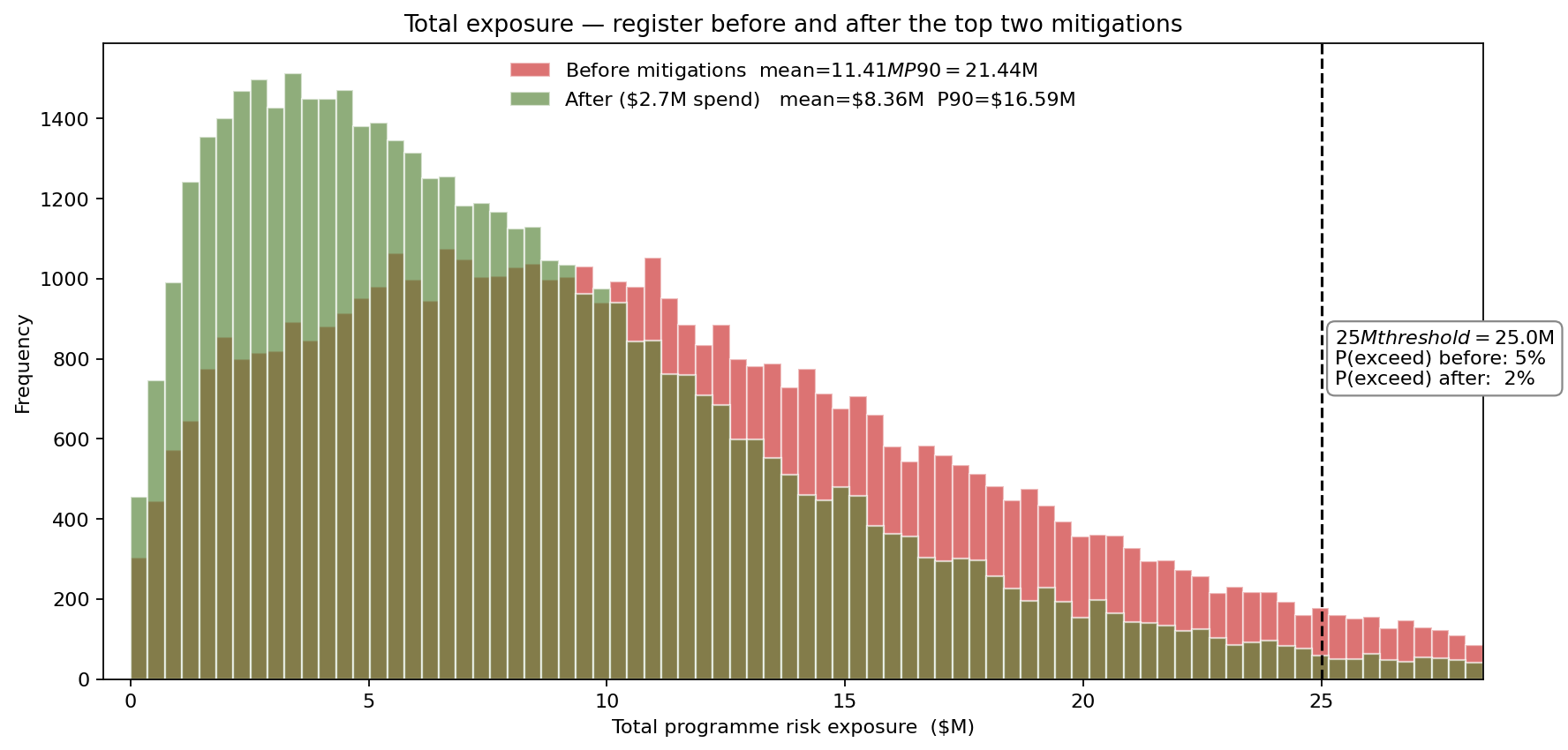
Combined, the two mitigations cost $2.7M up front and cut the P80 exposure from $17.2M to $12.7M — a $4.4M reduction at the 80th percentile — while pulling the mean down by $3.0M. On expected-value terms the $2.7M spend is essentially self-funding (roughly 1.1× the mean reduction), but the real case for it is the tail: it is the cheapest way to move the P80, and the chart, not the spreadsheet, was what got the steering committee to approve the spend.

Sensitivity: where the next mitigation dollar goes

A tornado over the P80 of total exposure ranked the residual drivers after the two top mitigations:

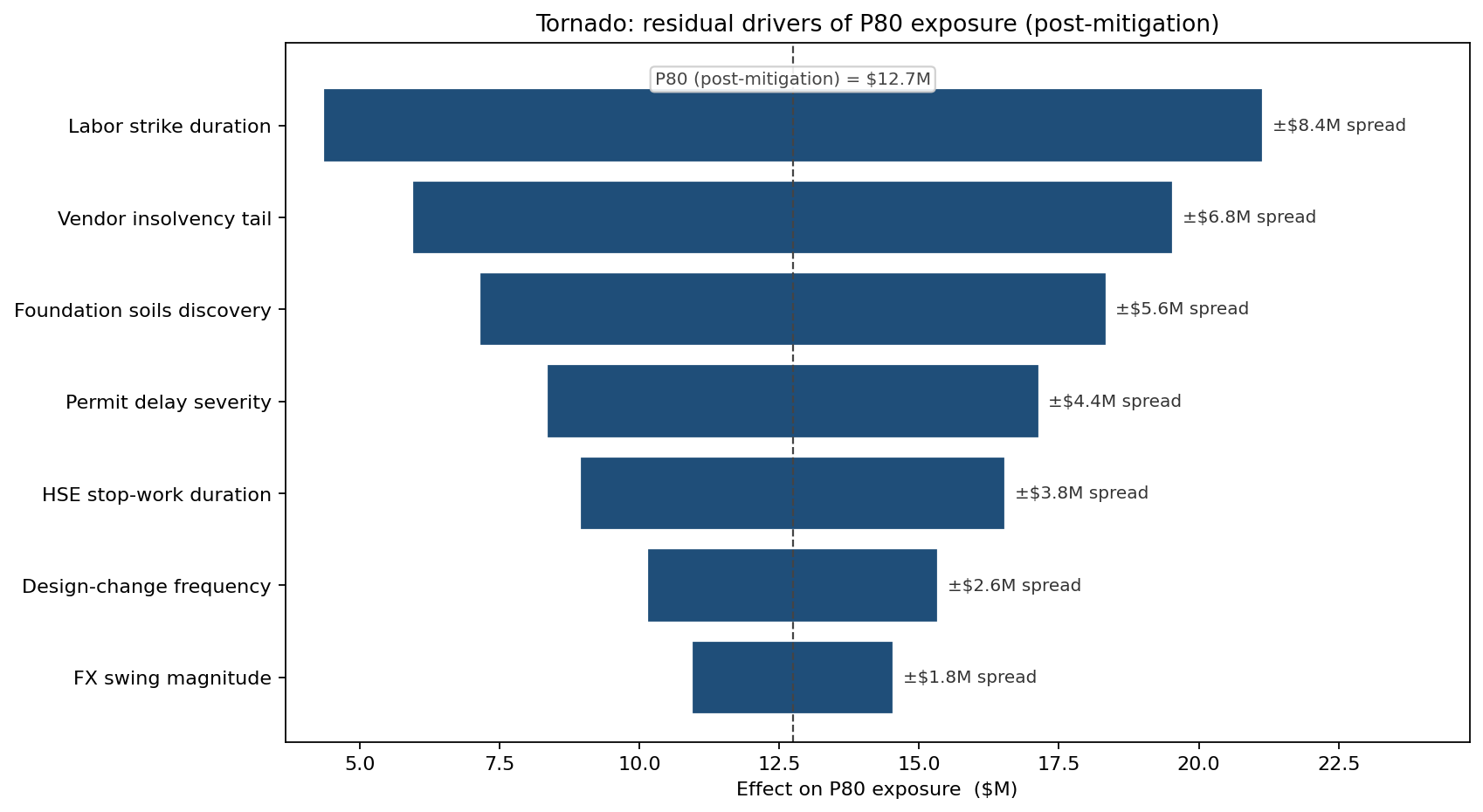
With the monsoon and customs risks reshaped, labor-strike duration moves into the top slot. That's the next mitigation conversation — likely a labor-agreement structure that caps the firing probability — and the tornado is the document that frames it.

What changed

• Contingency reset from $1.1M (10% of EMV) to about $5.8M (P80 minus mean), with the new figure defensible line-by-line to the board.
• $2.7M in concentrated mitigation spend (monsoon shelter + diversified supplier) cut the P80 exposure by $4.4M and the mean by $3.0M — the cheapest available way to move the tail.
• Register pruned from 47 lines to 12 actively managed lines representing the bulk of the exposure, freeing PM attention for the risks that actually move the number.

ModelRisk Functionality Used

• Beta(α, β) probability distributions on each register line — Beta(2, 18) for rare risks, Beta(5, 10) for credible risks — keeping the firing probability bounded on [0, 1] where Normal would not.
• LogNormal cost-impact distributions with mean = exp(μ + σ²/2), correctly capturing the right-tail behaviour of construction re-work and permit-driven cost shocks.
• Gaussian-copula common factors linking the firing of lines that share a root cause (weather window, regulatory cycle), so correlated risks co-fire in the same iterations and fatten the tail — an empirical firing correlation of ≈ 0.22 within the weather group rather than the asserted-but-absent dependence a naive register assumes.
• Pareto sort over expected impact that surfaced the 3-of-47 lines driving 56% of exposure, replacing equal-weight management attention with a prioritised list.
• Before/after re-simulation of the modified register that gave the steering committee a $4.4M P80 reduction figure with a chart, not a claim.

A risk register is a list; a risk register run through a simulation is a budget. Monte Carlo simulation in ModelRisk turns the register from "things we are worried about" into "the dollars we should be moving today, and the residual exposure that survives."