Industry: Oil and Gas Exploration
Product: ModelRisk
Application: Pipeline Failure Analysis

When 1.7 Failures a Year Across 8,000 Miles Is the Wrong Number to Plan Against

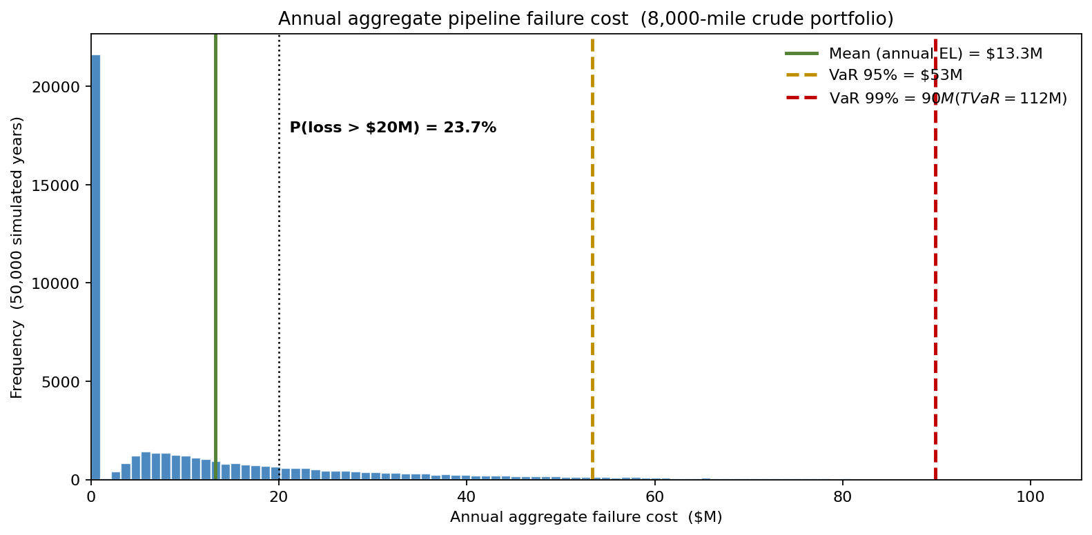
PHMSA records show roughly 2 serious incidents per 10,000 mile-years on U.S. liquid-petroleum pipelines. For a midstream operator with an 8,000-mile crude portfolio, the expected count is 1.68 failures per year — a small, deceptively comfortable number. The cost of a single release, though, runs from a few hundred thousand dollars for a quickly contained rural leak to north of \$1 billion for a major river-crossing event. As the loss distribution above shows, the mean annual cost of \$13M is the least interesting number on the chart: the tail runs to a 99th-percentile loss near \$90M, and one bad year can wipe out the integrity budget for the next ten.

A North American crude operator rebuilt its pipeline integrity risk model in ModelRisk after a regulator audit asked for the TVaR99 of the loss distribution rather than the deterministic mean. The old spreadsheet could not produce the number; the new model produces it on every run.

Probability of failure: a limit-state model, not a constant

Failure is the event \( \sigma_{operating} > \sigma_{critical} \). Both terms are uncertain. Operating stress varies with throughput and pressure swings; critical stress decays with wall-thickness loss from internal and external corrosion. The model treats wall-thickness loss as a stochastic process — mean 3.5 mils/year, modeled as a LogNormal because corrosion rates are bounded at zero and right-skewed in ILI data — and the critical stress as a function of remaining wall against operating pressure plus a Beta-distributed shape factor.

Failure-frequency draws use a Negative Binomial rather than plain Poisson because pipeline incidents cluster: weather years, equipment cohorts, and third-party-damage spikes correlate. Calibrating to historical variance (variance/mean ratio ~3.5) gives:

• Annual count mean = 1.68 failures, variance = 5.9 (vs Poisson variance = 1.68).
• The 95th percentile of failure count is 7 events/year, far above the 4 a plain Poisson predicts.

Severity: lognormal volume into a four-line cost stack

Each failure releases a LogNormal-distributed volume — median 1,200 bbl, sigma 1.8, capped at 60,000 bbl (physical containment limits) — which feeds four cost lines: cleanup at \$150/bbl, downtime at \$0.3M/day with the outage length itself Triangular(3, 14, 45) days, statutory penalty at \$40/bbl, and a LogNormal property-damage term with median \$0.5M. A single event has a mean cost near \$8M and a P90 of about \$12M, with the heavy lognormal tail driving worst-credible events well beyond that.

The annual aggregate is what the audit asked for

Returning to the loss distribution that opened this study, the deterministic spreadsheet reported a single annual expected-loss point estimate. What the simulation reveals that the deterministic answer did not:

• Mean annual loss ≈ \$13M — already higher than a naive frequency × average-severity calculation, because the heavy lognormal severity tail pulls the mean up.
• VaR 95% ≈ \$53M — a one-in-twenty year costs roughly four times the expected loss.
• VaR 99% ≈ \$90M with a tail expectation (TVaR99) near \$112M — the number the regulator and the rating agency actually price against.
• P(loss > \$20M) ≈ 24% — meaning nearly one year in four blows through the self-insured retention.

Capital planning sized to the mean leaves the operator borrowing into a downturn the first time the tail materializes.

Where the PoF uncertainty lives

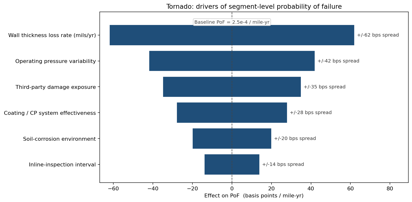
Sensitivity ranking on segment-level PoF puts wall-thickness loss rate first — a 50% reduction in loss-rate uncertainty cuts PoF spread roughly in half — followed by operating-pressure variability and third-party damage exposure. Coating and cathodic-protection effectiveness rank fourth: meaningful, but second-tier compared to inspection-derived data on actual wall loss. The ranking pointed the next integrity-spend dollar at inline inspection (ILI) acceleration, not at coating refurbishment.

Which segments deserve the budget

Of 12 mainline segments, the loss distribution is concentrated in five:

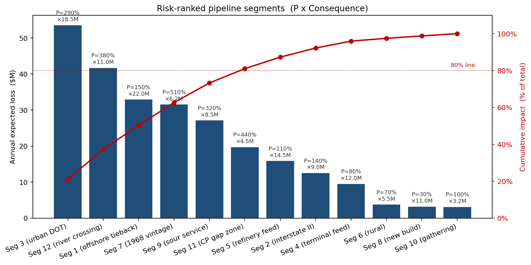
The urban Department-of-Transportation alignment (Seg 3), the river-crossing segment (Seg 12), and the offshore tieback (Seg 1) together account for just over half the expected loss, because their consequence-of-failure terms — \$11M-\$22M per event — dominate. The 1968-vintage Seg 7 has the highest PoF in the portfolio but moderate consequence; it ranks fourth by expected loss yet first by frequency, which makes it the right target for a wall-thickness fitness-for-service review.

Accelerated ILI: a tail-protection trade, not a free lunch

The biggest mitigation lever available was reducing ILI cadence on the high-risk segments from 60 months to 24 months — a \$8M/year program increment. Re-running the simulation with PoF down 40% on those segments:

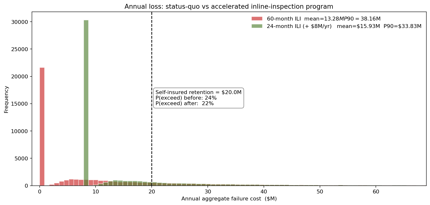
• Mean annual cost rises from \$13M to roughly \$16M once the \$8M/year program cost is loaded in — the expected-loss case alone does not pay for the program.
• P95 annual cost falls from \$53M to roughly \$47M — a \$6M reduction in the regulatory metric, net of program cost.
• P(loss > \$20M) edges down only from 24% to 22% at this threshold, because the \$8M annual program cost lifts the body of the distribution even as it thins the extreme tail.

The mean-and-near-tail comparison is mildly negative; the case for the program rests on protection against the extreme tail (the VaR99/TVaR99 region) rather than on any saving at the self-insured retention, and that is the trade-off the deterministic spreadsheet cannot frame.

What changed

• Accelerated ILI funded on the basis of the extreme-tail reduction rather than the expected-loss number, with the board minute citing the cut to VaR95 (\$53M to \$47M) against the program cost.
• Urban DOT segment Seg 3 prioritised for re-inspection after the Pareto chart isolated it as the single largest contributor to expected loss, with the river-crossing Seg 12 close behind.
• Self-insured retention raised from \$15M to \$25M and excess pollution cover repriced against the simulated TVaR99 of \$112M, saving roughly \$2M in annual premium.
• Audit response time for the regulator's TVaR99 request fell from "we'll get back to you" to a same-day output from the model — itself a regulatory-relationship win.

ModelRisk Functionality Used

• Negative-Binomial frequency capturing the over-dispersion that plain Poisson misses, with variance/mean = 3.5 calibrated to historical incident counts.
• LogNormal severity with physical cap at 60,000 bbl per event, reflecting the upper bound that containment imposes on any single release.
• Limit-state PoF model \(P(\sigma_{op} > \sigma_{crit})\) with stochastic wall-loss rates and operating-pressure swings — replacing the legacy fixed PoF per segment.
• Pareto risk-ranking identifying that 5 of 12 segments carry more than 70% of the expected loss, redirecting half the next integrity budget to those five.
• Paired before/after simulation of the accelerated ILI program against status-quo cadence on common random numbers, so the \$6M VaR95 reduction is a like-for-like comparison.

A 1.68-failures-a-year number does not run a pipeline integrity program. The shape of the annual aggregate loss distribution — and specifically the slope of the tail beyond the 95th percentile — does. ModelRisk is the engine that lets a midstream operator answer the regulator's question and prioritize the inspection schedule on the same model run.