

Industry: Oil and Gas
Product: ModelRisk
Application: Offshore drilling
When the Deterministic AFE Is Over-Run 58% of the Time: Probabilistic Well-Cost Modelling
A 6th-generation deepwater drillship dayrates at $550,000 per day, and once mud, downhole tools, services, and logistics are added, the all-in burn rate sits closer to $800,000 per day. For an 80-to-100-day well in 2,500 m of water, that is the difference between a $96M well and a $128M well — entirely on the schedule, before any reservoir uncertainty enters the picture. The conventional Authorization for Expenditure (AFE) computes a single number from phase-average durations plus a flat 7-day NPT (non-productive time) contingency. Across a 12-well deepwater campaign, a deterministic AFE typically over-runs in half or more of all wells — a coin-flip-or-worse outcome that the AFE document presents as a defended estimate. A deepwater operator rebuilt the AFE process in ModelRisk as a full probabilistic schedule-and-cost model. The single chart that reframed the capital conversation overlays the full cost distribution on the deterministic AFE:
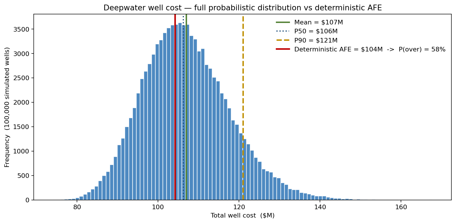
The deterministic AFE (~$104M) lands just below the simulated median, and the realised well cost exceeds it about 58% of the time — the over-run risk a single AFE number presents as a defended estimate. The sections below build that distribution from its phase and non-productive-time drivers.
The phase stack and its distributions
Five operating phases, each with a distribution that matches its physical character:
| Phase | Distribution | Mean (days) | P90 (days) |
|---|---|---|---|
| Mob & site setup | Triangular(8, 12, 25) | 14 | 21 |
| Surface 13-3/8" csg | LogNormal(μ_mean=18, σ=5) | 18 | 25 |
| Intermediate 9-5/8" csg | LogNormal(μ_mean=22, σ=7) | 22 | 31 |
| 7-in liner | LogNormal(μ_mean=16, σ=6) | 16 | 24 |
| Logging & completion | LogNormal(μ_mean=14, σ=5) | 14 | 21 |
Triangular for mob, where the geometry is bounded and the mode is well-elicited. LogNormal for everything downhole, because operating phases are positively skewed — most go to plan, a few have hole-instability or directional-trouble surprises that double the time. Using Normal here, as several in-house cost models do, lets the simulator draw negative durations and erases the upside tail that defines AFE risk.
Four sources of non-productive time, each with its own probability law
The flat 7-day NPT contingency in the deterministic AFE is the second large source of bias. The simulation replaces it with four physically distinct sources:
- BOP test failures. Each well requires four blowout-preventer pressure tests; each test has a Bernoulli failure probability of 18% (post-Macondo regulator stats). Each failure costs LogNormal(mean 3 d, σ 1.5 d) to remediate.
- Stuck pipe. Bernoulli 8% per phase across four downhole phases. Each event costs LogNormal(mean 5 d, σ 3 d). The longest tail in the simulation.
- Weather waiting. Poisson 1.5 events per well under in-season operations (waiting on Hs > 4 m). Each wait LogNormal(mean 2.5 d, σ 1.5 d).
- Misc downhole / service. Smaller contributor, captured as residual.
Aggregate NPT has mean roughly 7.5 days, P90 ≈ 15 days, with a tail extending to 30+ days driven by the rare double-stuck-pipe events.
The cost distribution
Reading the distribution above against the AFE line gives the numbers the capital committee actually needs. The deterministic AFE comes in at approximately $104M (89 days × $800k/day + $33M tangibles/mob). The simulation produces:
- P50 ≈ $106M — close to the AFE, as expected
- Mean ≈ $107M — above P50 because the cost distribution is right-skewed (the sum of right-skewed phase distributions plus a right-skewed NPT compound process)
- P90 ≈ $121M — a 14% headroom over P50 that the AFE-plus-contingency cannot match
- P(cost > AFE) ≈ 58% — worse than a coin flip, the over-run risk the deterministic AFE hides
The chart is the indictment of single-number AFE management: the deterministic AFE sits just below the median, not at a defensible upper bound. A capital plan that allocates only the AFE amount is under-funded in well over half of all wells. A campaign of 12 wells funded on AFE has a >95% probability that aggregate cost exceeds aggregate AFE.
Where the days actually live
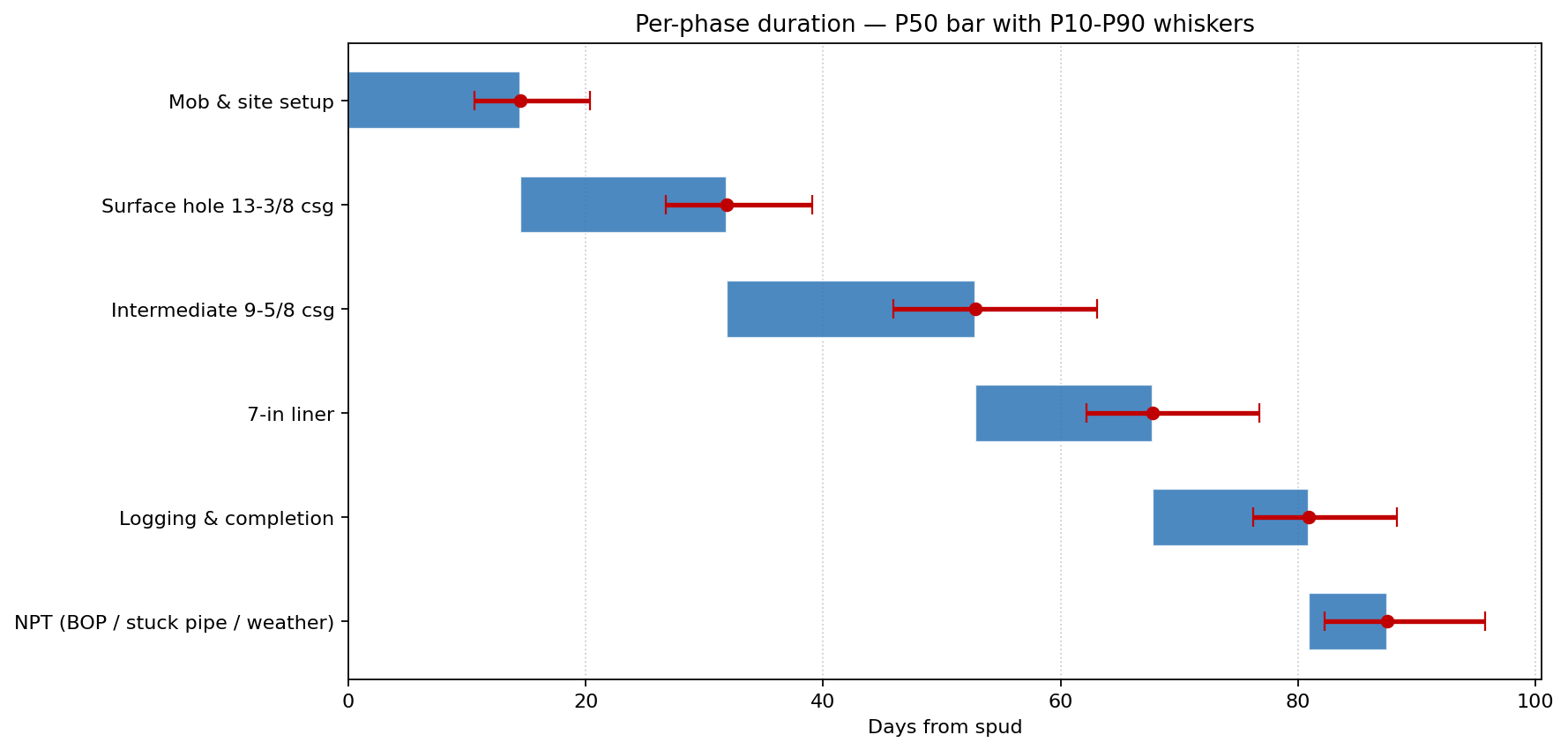
The Gantt-style chart shows each phase's median duration with P10–P90 whiskers — the visual that immediately tells the drilling superintendent where the schedule risk concentrates. The 9-5/8" intermediate casing phase has the widest P10–P90 spread (largest single attackable risk), and the aggregated NPT bar has the longest absolute spread of all — confirming that operational reliability investments dominate engineering-phase optimisations.
What actually drives the cost
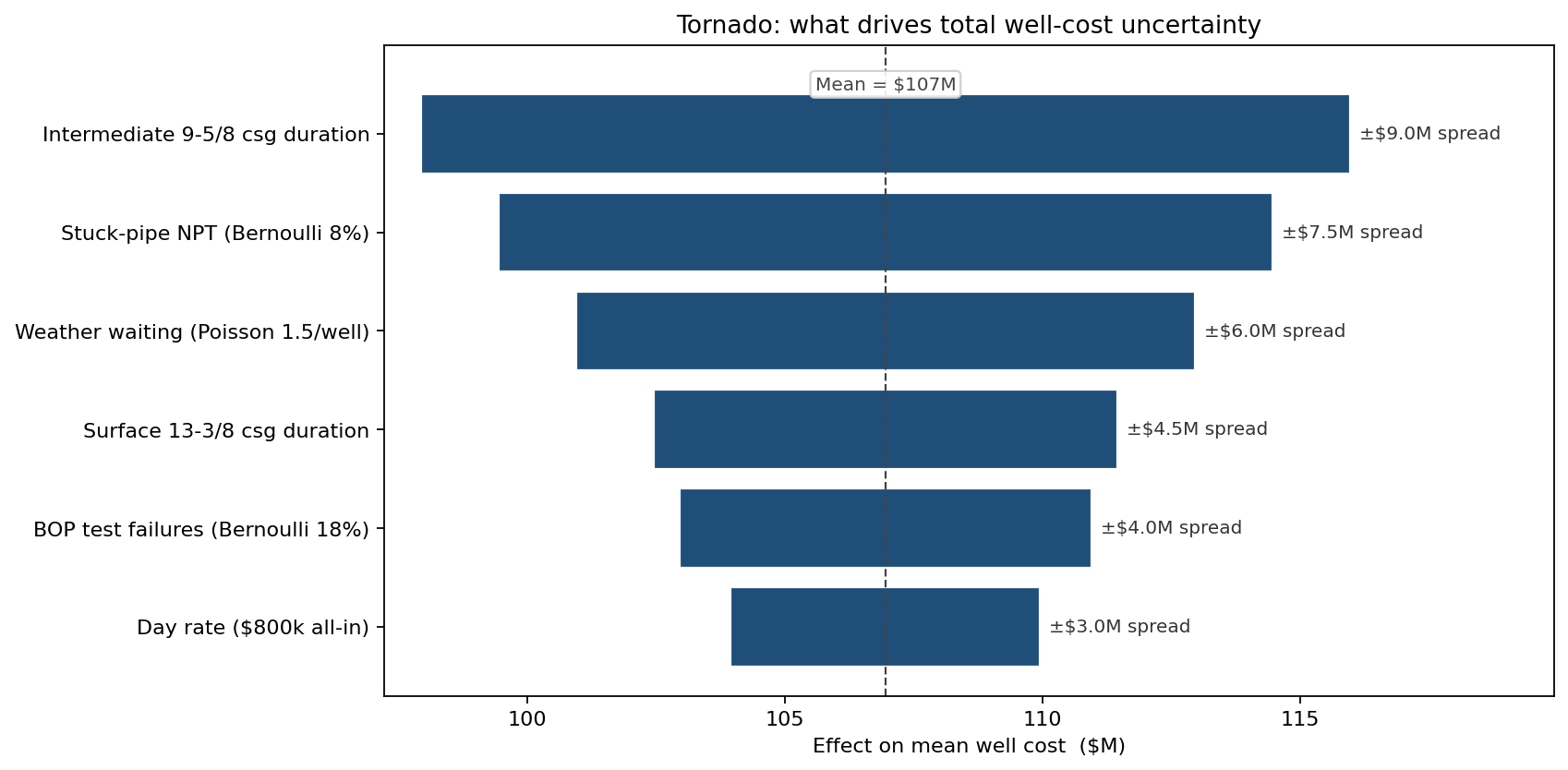
The intermediate-casing phase dominates by absolute spread (single largest phase, widest LogNormal). Stuck-pipe NPT ranks second, and the implication is operational: investing in real-time drilling-data analytics, automated stuck-pipe early-warning systems, and best-in-class mud programs pays back faster than any phase-engineering optimisation. Weather waiting ranks third — modest individually, but big in aggregate during winter campaigns. The dayrate itself ranks last among the top drivers, because while it is a large absolute number it is a known constant; the variance it contributes is zero.
What changed
- AFE process replaced by P50 / P90 budgeting. The capital approved per well is the P70 cost ($112M) rather than the deterministic AFE — a roughly 7% uplift that brings the over-run probability from 58% down to 30%, the corporate risk-appetite target.
- Contingency reserve sized at fleet level rather than per well. Pooling 12 wells' tail risk via the simulation showed that a single $40M campaign-level contingency outperforms 12 individual $5M contingencies — the same diversification logic that insurance applies to claims.
- Stuck-pipe analytics investment funded at $2.5M one-time, justified by the simulation showing it cut the stuck-pipe Bernoulli from 8% to 4%, worth ~$1.5M expected savings per well or $18M across a 12-well campaign.
- Rig contract renegotiated with a performance-incentive clause tied to actual days under P50 — using the simulation as the shared baseline rather than the disputed deterministic AFE.
- Weather window for two wells in the campaign deferred to summer based on the Poisson rate doubling in winter; net cost saving estimated at $4M per deferred well.
ModelRisk Functionality Used
- Phase-by-phase distribution stack — Triangular for the bounded mob phase, LogNormal with method-of-moments fit for each downhole phase — replacing the single-AFE-number-plus-contingency that erases the right tail.
- Compound NPT model with Bernoulli (BOP tests, stuck pipe), Poisson (weather), and LogNormal severities — the right mixture of frequency-severity processes for events that are physically distinct.
- Stochastic Gantt visualisation with P10/P50/P90 whiskers per phase, the chart the drilling superintendent uses to prioritise attention to high-variance phases.
- Aggregate-cost histogram with deterministic AFE overlay, making the P(cost > AFE) ≈ 50% finding visible to the capital committee in a single chart.
- Tornado sensitivity ranking the stuck-pipe Bernoulli as the highest-leverage attackable risk — directly funding the real-time analytics investment that the deterministic AFE could not justify.
- Campaign-level aggregation via re-sampling 12 wells per simulation run, producing the fleet-level contingency calculation that pools the tail risk.
The deterministic AFE is not a budget; it is a 50/50 bet. Monte Carlo simulation in ModelRisk replaces that bet with the P70 budget management actually approves and the operational priorities the budget actually depends on — a discipline difference far larger than any per-phase engineering optimisation.