Industry: Oil and Gas
Product: ModelRisk
Application: Energy trading

Why Flat-Vol GBM Underprices Oil and Gas Tail Risk: VaR for a Crude + Gas Trading Book

The chart below is the one the chief risk officer needs to see. It overlays two 10-day P&L distributions for the same trading book, simulated with the same diffusion volatility and the same WTI-Brent correlation. The only difference is the price process: a flat-volatility geometric Brownian motion (the textbook default) versus a mean-reverting Schwartz one-factor model with Poisson jumps.

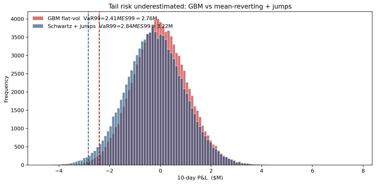
The two distributions agree through the body and diverge in the left tail. The flat-vol GBM reports a 10-day VaR 99% of about $2.41M; the jump model reports $2.84M — a 15% understatement of the regulatory capital charge, concentrated entirely in the discrete jump mass that a Gaussian tail cannot hold. WTI dropped $9/bbl in a single April 2020 session, and Henry Hub natural gas printed daily moves of 25% during the February 2021 Texas freeze; those are the moves living in that tail. The trading risk team rebuilt their value-at-risk engine in ModelRisk around the Schwartz-plus-jumps process, calibrated separately for crude and for natural gas, on a book holding 500,000 barrels of WTI long against a 480,000-barrel Brent short hedge plus one million MMBtu of Henry Hub length.

Why GBM is the wrong process for commodities

Geometric Brownian motion has two properties that crude oil and natural gas demonstrably do not share: log-returns are independent (no mean reversion), and there are no jumps. Both assumptions fail empirically. The marginal cost of producing the last barrel of US tight oil acts as a soft floor around $40–50/bbl; OPEC quota discipline acts as a soft ceiling above $90. Prices wander but return to an equilibrium band on a roughly six-month half-life. Natural gas mean-reverts even harder — the half-life of Henry Hub deviations from the storage-implied forward curve is closer to three months — but is also far more jump-prone, with weather and pipeline outages producing daily moves the lognormal tail cannot accommodate.

The model used here is log-price Ornstein-Uhlenbeck with a compound Poisson jump:

\[ d\ln S_t = \kappa(\ln\theta - \ln S_t)\,dt + \sigma\,dW_t + J\,dN_t \]

For WTI: equilibrium θ = $70/bbl, mean-reversion speed κ = 1.5/yr, diffusion volatility σ = 38% annual, jump intensity λ = 8/yr with mean jump −9%, jump-size standard deviation 12% — sized to the single-session gaps crude actually prints. For Brent the same structure with θ = $74 and a correlation ρ = 0.93 to WTI on the diffusion shocks plus 92% jump co-arrival — the inter-grade basis is tight but not perfect. For Henry Hub: θ = $3.20/MMBtu, κ = 2.5/yr, σ = 55%, λ = 14/yr with mean jump −12% and standard deviation 22% — a higher jump rate and far fatter jumps than crude, because gas storage runs out faster than crude inventory does and weather shocks are violent.

The 10-day P&L distribution

The simulation runs 100,000 correlated 10-day paths for the three benchmarks and revalues the book at horizon. The starting marks are WTI $72, Brent $76, Henry Hub $3.40/MMBtu. The mean P&L is approximately zero (the desk is roughly market-neutral after the hedge). The distribution looks like this:

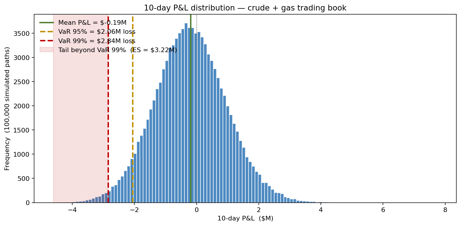
The 10-day VaR 99% is approximately $2.84M and the expected shortfall in the tail beyond VaR 99% is roughly $3.22M. The flat-vol GBM with matched diffusion volatilities and no jumps produces a VaR 99% of about $2.41M — a 15% under-statement of the regulatory capital charge. The shape of the difference is the tail: GBM puts negligible mass in the extreme jump-driven losses, while the Schwartz-plus-jumps process carries a visible fat left tail that drives both the higher VaR and the wider gap in expected shortfall.

What actually drives the VaR

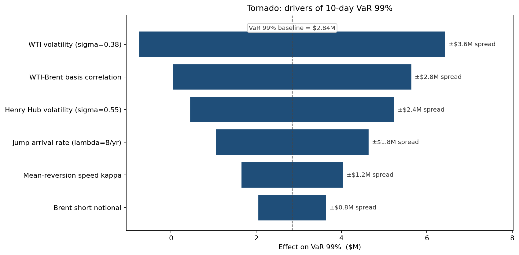
WTI volatility is the largest driver — unsurprising for the largest single position. The WTI-Brent correlation is second, because the hedge ratio is leveraged on this number: at ρ = 0.93 the WTI long is well-hedged, at ρ = 0.85 the residual basis exposure adds significantly to VaR. Henry Hub volatility is third — the position is smaller but the per-MMBtu volatility is much higher. The jump intensity λ matters more in expected shortfall than in VaR 99%: ES is more sensitive to the tail shape, VaR to the body.

The picture the desk presents to the risk committee

The overlay shown at the top of this article is the chart the desk takes to the risk committee every quarter. Two distributions with the same diffusion volatility produce VaR 99% numbers that differ by roughly 15%, and that gap is the regulatory capital requirement underestimation. Reporting the GBM number and being told by a regulator that the backtest fails (too many exceedances over the last 250 days) is the predictable consequence the jump model fixes.

What changed

• Regulatory VaR rebenchmarked: the official VaR 99% moved up by approximately $0.43M (from $2.41M to $2.84M), with the corresponding capital reserve allocated honestly rather than discovered after a model breach.
• Hedge ratio recalibrated: the WTI-Brent hedge was tightened from 0.92 to 0.96 after the simulation showed the residual basis exposure was the second-largest single driver of VaR.
• Henry Hub position sized down by 15% during winter weeks when the model's jump component is active, freeing risk-budget for the higher-Sharpe crude relative-value trades.
• Backtest exceedances dropped from 6/250 days under the GBM model to 3/250 days under the jump model — within the 99% confidence band rather than triggering the Basel traffic-light yellow zone.
• Calendar-spread option pricing reused the same paths, producing internally consistent prompt vs deferred volatility surfaces.

ModelRisk Functionality Used

• VoseTimeSeries with mean-reverting Schwartz for WTI, Brent, and Henry Hub, parameterised separately rather than using the default GBM that turns up in commodities textbooks but fails empirical backtests.
• Compound Poisson jumps layered on the diffusion, with separate intensities for oil (λ = 4/yr) and gas (λ = 8/yr) calibrated to the historical frequency of >5% daily moves.
• Cross-grade correlation via shared Brownian increments (ρ = 0.93 WTI-Brent diffusion) plus co-arriving jumps — capturing the empirical fact that crude grades move together in both normal and stressed regimes.
• Custom revaluation formulas for the book at horizon — physical crude positions plus a 1M-MMBtu Henry Hub futures stack — all evaluated inside Excel against live position blotters.
• VaR / ES outputs in the format the Basel regulatory submission accepts, including 250-day backtest tracking.
• Side-by-side overlay of GBM and the chosen process, which is the chart the desk uses every quarter to justify the model-selection choice to the model risk committee.

The choice of price process is not a modelling detail — it is the difference between a VaR number a regulator will accept and one they will reject. Monte Carlo simulation in ModelRisk lets the trading desk run the right process, not the convenient one, and report a VaR that holds up to backtest scrutiny.