Industry: Oil and Gas
Product: ModelRisk
Application: Drilling risk analysis

When the High-Volume Prospect Is the Wrong Bet: Probabilistic Drilling Risk Analysis

A single deepwater exploration well in the pre-salt offshore Brazil costs $120 million to drill and another $30 million in rig mobilisation and seismic — and the historical wildcat success rate in frontier deepwater plays sits between 25% and 45%. On a portfolio of six prospects evaluated each year, deterministic ranking by mean recoverable volume routinely pushes capital into the worst risk-adjusted bets. A pre-salt operator rebuilt its prospect ranking in ModelRisk to replace single-number Pg and P50-volume comparisons with full Expected Monetary Value (EMV) distributions per prospect.

The result is the chart that a single EMV number can never show: a genuinely bimodal outcome — a heavy dry-hole branch on the left and a long success tail on the right — for one deepwater prospect.

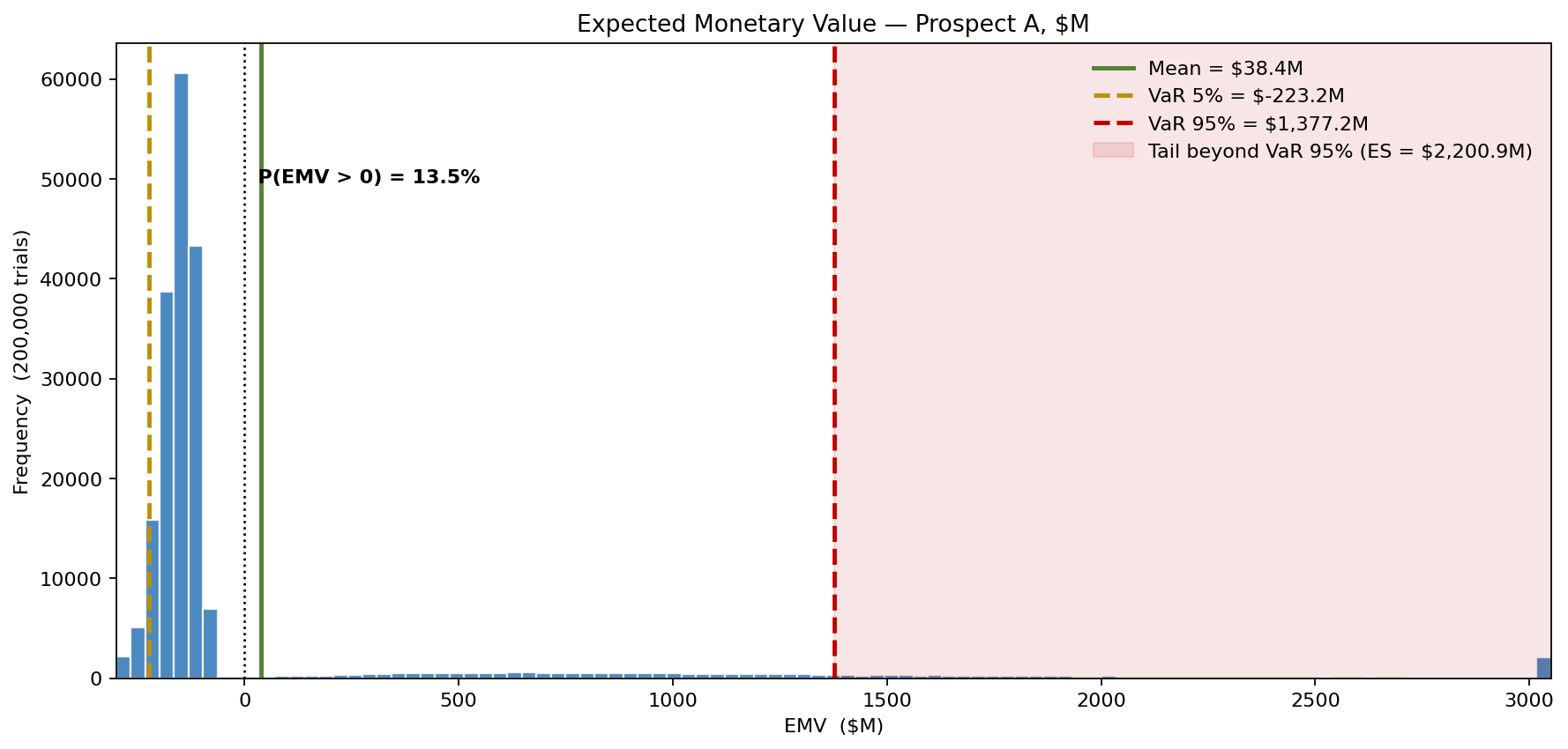
The simulation reveals roughly an 86% probability that the realised outcome is a dry-hole loss of $80–$220M and a 14% probability of a $300M–$3B gain. The mean EMV is genuinely positive (+$50M), but the dry-hole probability is the headline that the deterministic +$60M point estimate buries. The sections below build that distribution layer by layer.

The chance-of-success calculation that point estimates corrupt

The chance of geological success multiplies four independent factors — trap, reservoir, seal, and charge — each elicited from geoscientists as a Beta distribution rather than a single number. For Prospect A (a deepwater Santos Basin lead), the central estimates were P(trap) = 0.60, P(reservoir) = 0.70, P(seal) = 0.50, P(charge) = 0.67. A naive multiplication gives Pg ≈ 0.14. The Monte Carlo result tells a richer story: the Pg distribution itself has P10 = 0.06 and P90 = 0.23 — the spread that the single product hides. Treating Pg as deterministic when its 10th-to-90th-percentile range spans an order of magnitude is the most common single error in exploration economics.

\[ Pg = P_{trap} \times P_{reservoir} \times P_{seal} \times P_{charge} \]

Volume given success: lognormal product, not normal sum

Recoverable volume is the product of six physical parameters — area, net pay, net-to-gross, porosity, hydrocarbon saturation, and recovery factor. Because the product of positive variables is approximately lognormal (central limit theorem on logs), the volume distribution is right-skewed and the mean sits well above the median. Modelling each input as LogNormal in ModelRisk yields, for Prospect A, a recoverable volume with P50 ≈ 110 MMboe, mean ≈ 130 MMboe, P90 ≈ 225 MMboe. Reporting the P50 as "the" volume understates expected value; reporting the mean overstates median outcome. The full distribution is what feeds NPV.

From volume to NPV: oil price as mean-reverting equilibrium, not GBM

Long-horizon oil-price modelling using geometric Brownian motion is a common but indefensible choice — Brent does not have an exponential trend over 20 years, it mean-reverts to a marginal-cost equilibrium punctuated by structural breaks. The simulation treats realised average Brent over the producing life as a wide distribution centred on $70/bbl with stress to $30 and $130, reflecting the regimes of 2014–16 and 2022. Per-boe post-tax PV is built from price minus 30% government take minus $18/boe development capex minus $12/boe lifting cost, all run through a present-value factor of 0.55 calibrated to the 18-year production profile at 8% discount. The mean discounted netback is $10.1/boe, with P10 of $3/boe and P90 of $17/boe.

Where the EMV distribution lives

The Expected Monetary Value combines Pg, NPV given success, and the dry-hole loss:

\[ EMV = Pg \times NPV_{success} + (1 - Pg) \times NPV_{failure} \]

For Prospect A, dry-hole cost is LogNormal centred on $150M (deepwater rig + mobilisation + abandonment). Per-iteration the simulation draws Pg, draws the volume and price stack, then draws a Bernoulli outcome to decide whether the well succeeds. That mechanism is what produces the bimodal EMV distribution shown above — the dry-hole branch and the success branch are separate populations, not a smear around a single mean. The deterministic EMV from point estimates is +$60M, comfortably positive; the simulation mean is +$50M. For a single-well decision, the dry-hole probability is the headline. Across a 10-well portfolio, the mean matters.

What actually moves the EMV

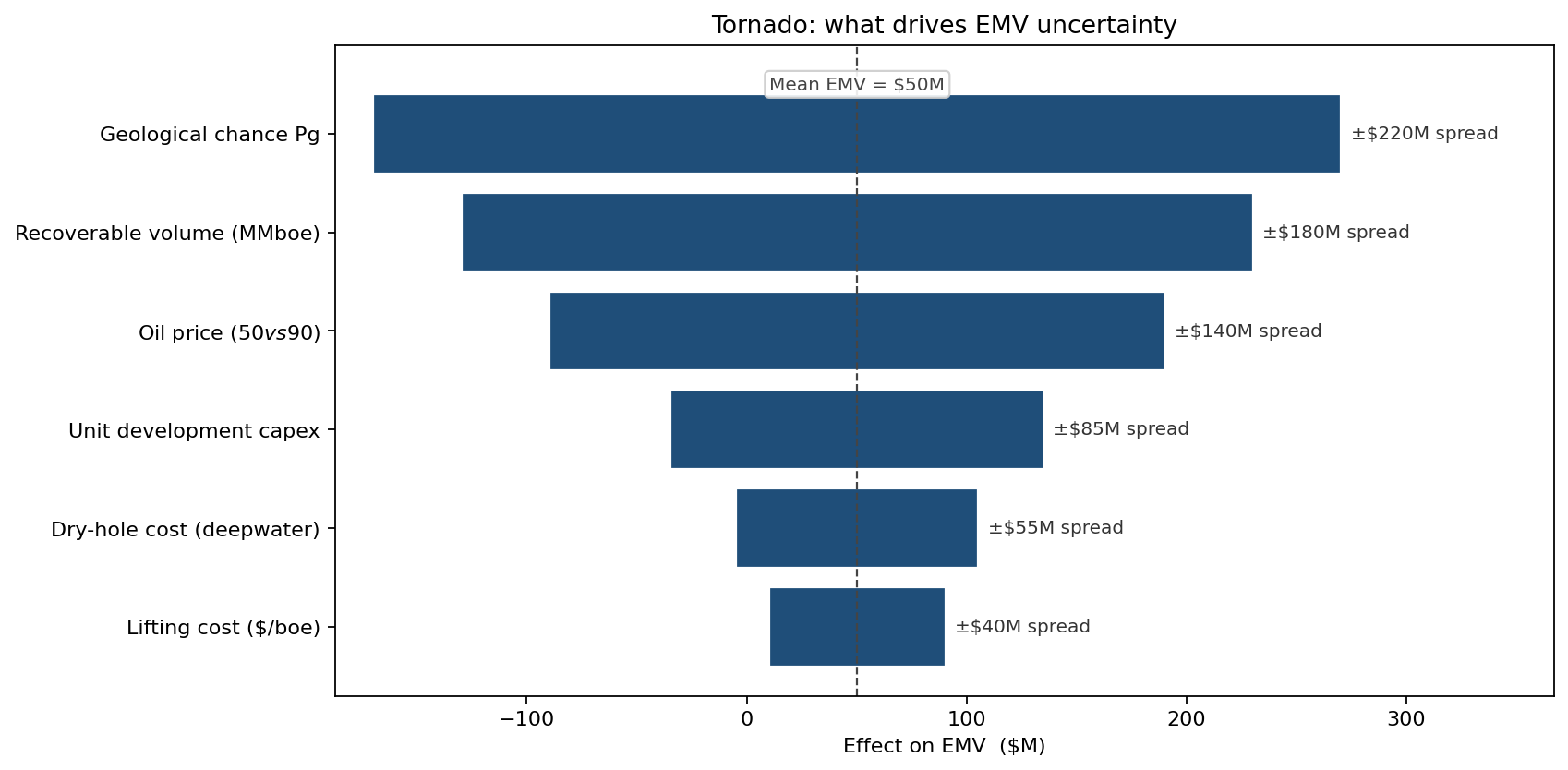
Pg ranks first — by a wide margin — and that ranking is itself the prioritisation: an additional 2D seismic program that tightens Pg from a [0.06, 0.23] range to a [0.10, 0.18] range is worth more than a 10% reduction in unit capex. Volume uncertainty is second, justifying further well-log reprocessing on offset wells. Oil-price uncertainty is third — large in absolute dollars but harder to attack from inside the exploration team. Unit capex and dry-hole cost trail, but show up large enough that the drilling-engineering function gets a quantified seat at the prioritisation table.

Prospect A vs Prospect B: the high-volume bet is the wrong bet

The most consequential application was head-to-head ranking of Prospect A (deepwater, big, low Pg) against Prospect B (shelf, smaller, higher Pg):

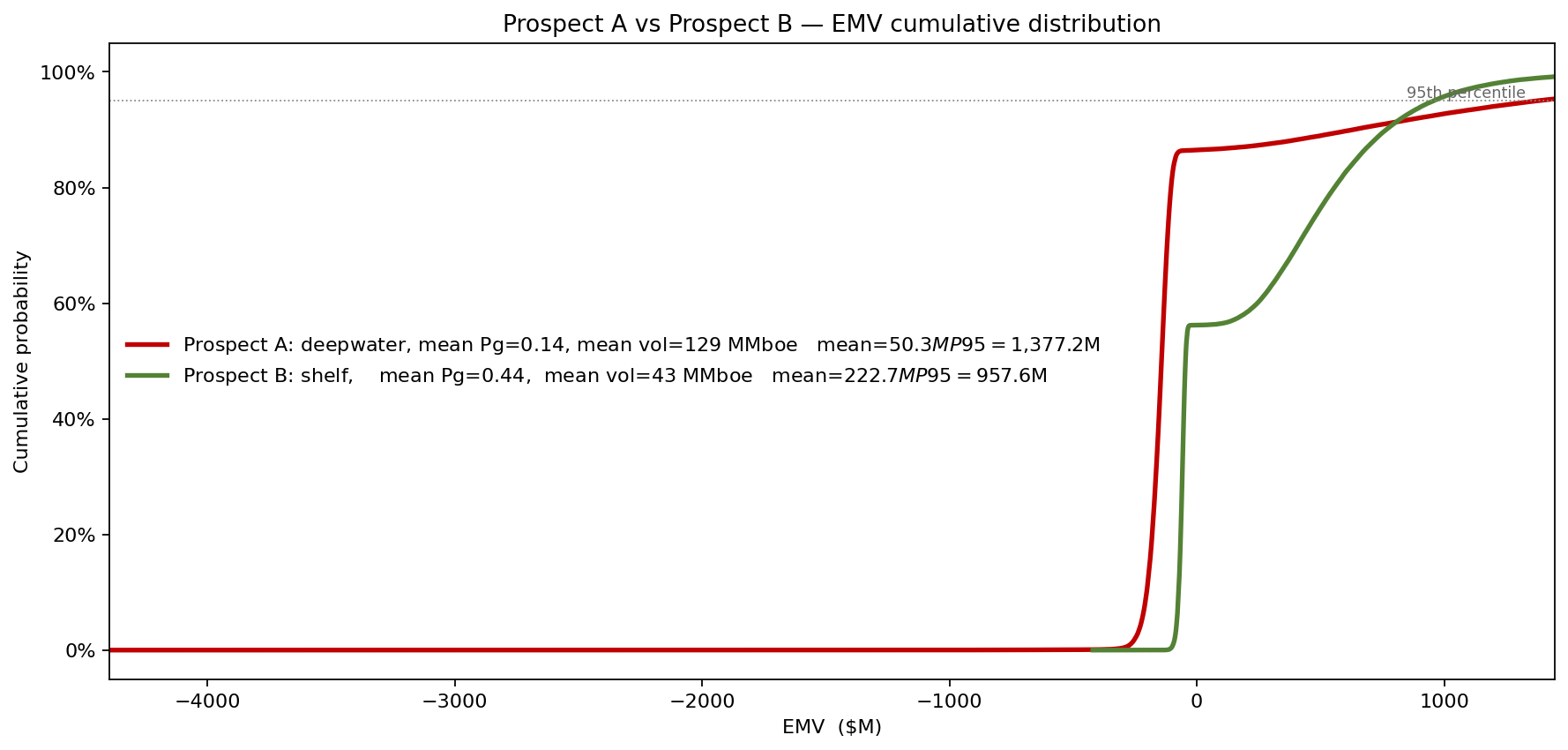
Deterministic ranking by mean volume × Pg × $10/boe put Prospect A first. The probabilistic ranking reverses the order. Prospect B has a much higher Pg (~0.44) and a much smaller dry-hole cost ($60M vs $150M), so its EMV distribution carries a far higher mean — +$223M versus Prospect A's +$50M — even though its smaller reserves mean it still drills a dry hole about 56% of the time. The decisive difference is the downside: Prospect B's loss is bounded by the cheaper well cost (P10 ≈ −$74M), while Prospect A compounds a $150M dry-hole loss with the rig-mobilisation sunk cost (P10 ≈ −$203M, with a P50 below zero). The high-volume prospect loses more, more often, when it loses.

What the model changed

• Capital reallocated from Prospect A to Prospect B for the current drilling slot; Prospect A was deferred pending an additional 3D seismic survey costing $8M — paid for many times over by the avoided dry-hole probability.
• Pg uncertainty became a tracked KPI rather than a single number filed in the prospect dossier. Geological reviews now report P10/P50/P90 Pg.
• Portfolio-level EMV stacking showed that a six-well 2024 programme had a 22% probability of negative aggregate EMV — a number the deterministic sum did not produce. Two of the six prospects were demoted to "watch" status.
• Reserves report consistency: P10/P50/P90 reserves now flow from the same simulation that produced EMV, eliminating the inconsistency between the petrophysics team's volumes and the economics team's NPV inputs.

ModelRisk Functionality Used

• Beta-product chance factors for trap / reservoir / seal / charge, with the Pg distribution itself an output and reported with P10–P90 rather than as a single point.
• LogNormal volumetric stack with each of the six volume factors as an independent draw, producing the right-skewed reserves distribution the linear formula cannot.
• Mean-reverting oil-price distribution centred on $70/bbl with the simulator drawing realised averages from $30 to $130 — replacing the GBM-on-Brent default that does not match a mean-reverting commodity.
• Bernoulli on Pg per iteration so the EMV histogram is genuinely bimodal (dry-hole branch vs success branch), exposing the loss-probability that the EMV mean alone hides.
• Tornado sensitivity ranking Pg, volume, and price as the top three EMV drivers — directly funding the next seismic / petrophysics / hedging investment decision.
• Side-by-side CDF comparison of competing prospects, the chart the exploration committee uses to allocate the year's drilling slots.

In exploration, the high-volume prospect is often the wrong bet — and the deterministic EMV is exactly the metric that hides why. Monte Carlo simulation in ModelRisk turns "rank by mean" into "rank by distribution," and that is the difference between a portfolio that survives the dry-hole years and one that does not.