

Industry: Manufacturing
Product: ModelRisk
Application: Supply Chain Bottleneck Identification and Mitigation
Why the $4.2M Dual-Sourcing Project Did Not Move Fill Rate: A Five-Component JIT Simulation
A consumer-electronics OEM was hitting only 88.5% fill rate against a 95% customer commitment — missing the target in essentially every year — and writing off $14.2M of annual revenue to stockouts. The executive playbook was clear: dual-source the single-source SoC at a $4.2M annual premium, because semiconductor disruption was the headline risk. The supply-chain finance team rebuilt the five-component JIT chain as a Monte Carlo simulation in ModelRisk before signing the dual-source contract. The simulation said: dual-sourcing the SoC alone barely moves the annual revenue loss at all — from $14.17M to $14.13M. The real bottleneck was not disruption, it was the LogNormal tail of routine lead time on the thinly-buffered components, and the cheapest fix was 50% more safety stock at $1.8M/year, which cut the annual loss to $4.85M.
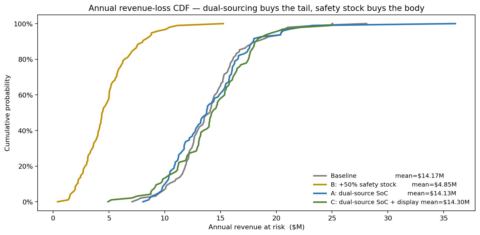
Three of the four annual-loss curves — baseline, dual-source SoC, and dual-source SoC-plus-display — are visually indistinguishable. Only the safety-stock strategy moves. That single chart is the whole story: the headline risk and the dominant risk were not the same component.
A JIT chain has two failure modes, not one
The chain has five gating components: display panel, SoC, battery cells, PCB assembly, and mechanical enclosure. Weekly demand is approximately Normal(8,500, 1,100) units. Production each week is constrained by the minimum on-hand of any of the five components — a stockout of any one halts shipment of all. Two distinct stochastic processes determine on-hand stock:
- Routine lead-time variability. Lead time is LogNormal per component — SoC mean 14 weeks (σ_log = 0.22), display 9 weeks (0.18), battery 6 weeks (0.25), PCB 5 weeks (0.20), enclosure 7 weeks (0.15). LogNormal because the body of the distribution is concentrated near the mode but the right tail is long — orders normally arrive within ±1 week of plan, but the worst 5% of orders arrive 4–6 weeks late.
- Disruption events. Independently each week, a component faces a low-probability disruption — port closure, fab fire, geopolitical event — that adds 4–12 extra lead weeks. Probability per week per component is 0.5–1.2% (single-source) or 0.4–0.6% (dual-source).
Safety stock is held in weeks-of-demand per component (SoC 4.5 wk, display 3.0 wk, battery 2.0 wk, PCB 1.8 wk, enclosure 2.0 wk). Re-orders are placed weekly to a target of (mean LT + safety weeks) × demand.
What the deterministic spreadsheet says vs what 5,000 weeks of simulation show
The deterministic planner using mean lead times and mean demand reports a 99%+ fill rate and zero meaningful revenue loss. The Monte Carlo over 5,000 weeks (~96 production years) tells a different story.
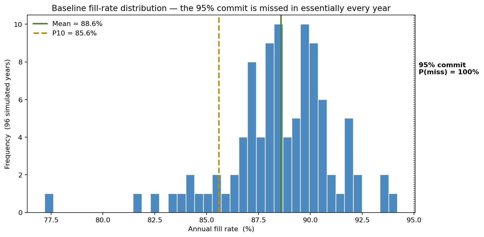
Mean annual fill rate 88.5%, P10 85.6%, weeks-with-shortage 27%, and the 95% commit is missed in essentially every simulated year. Mean weekly shortage 974 units. At $280 contribution margin per unit not shipped, that compounds to $14.2M/year in mean revenue at risk, with P90 = $18.2M. The deterministic spreadsheet missed this entirely because it averaged out the routine lead-time tail.
Where the executive's intuition was wrong
The instinct was that disruption events on the single-source SoC were driving the shortage. The simulation says otherwise: routine LogNormal lead-time tail variability dominates the disruption tail by roughly 4-to-1. The disruption tail is rare and dramatic; the routine tail is frequent and just-as-painful, and it is the routine tail that hits the safety-stock buffers week after week.
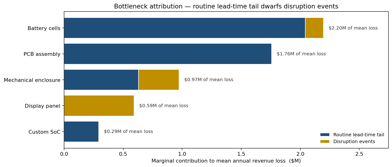
The attribution analysis quantifies the marginal contribution of each component to expected revenue loss, split into two channels: collapse a component's disruption probability to zero (the disruption channel), then also collapse its routine lead-time variability to deterministic (the routine channel). Two findings invert the executive's intuition. First, summed across the chain, the routine channel ($4.7M) is roughly 4× the disruption channel ($1.1M) — routine lead-time tails, not catastrophic events, drive the loss. Second, the binding components are not the SoC and display at all: they are battery cells (~$2.2M) and PCB assembly (~$1.8M) — the components with the thinnest safety-stock buffers (2.0 and 1.8 weeks). The well-buffered SoC contributes ~$0.3M and its disruption channel is essentially zero. The dual-source contract was a $4.2M/year insurance premium against a near-zero hazard.
Three strategies, one CDF, an inverted ranking
| Strategy | Mean loss ($M) | P90 loss ($M) | Cost ($M/yr) | Net ($M/yr) |
|---|---|---|---|---|
| Baseline | 14.17 | 18.17 | 0 | -14.17 |
| A: dual-source SoC | 14.13 | 17.93 | 4.2 | -18.33 |
| B: +50% safety stock everywhere | 4.85 | 8.03 | 1.8 | -6.65 |
| C: dual-source SoC + display | 14.30 | 18.16 | 6.8 | -21.10 |
The CDF makes the inversion vivid. Strategy B's curve sits far to the left of A and C across the entire distribution. Dual-sourcing buys protection against the rare tail; safety stock buys protection against the everyday body. With this chain's risk structure, the everyday body is where the money is.
The trade-off chart that ended the debate
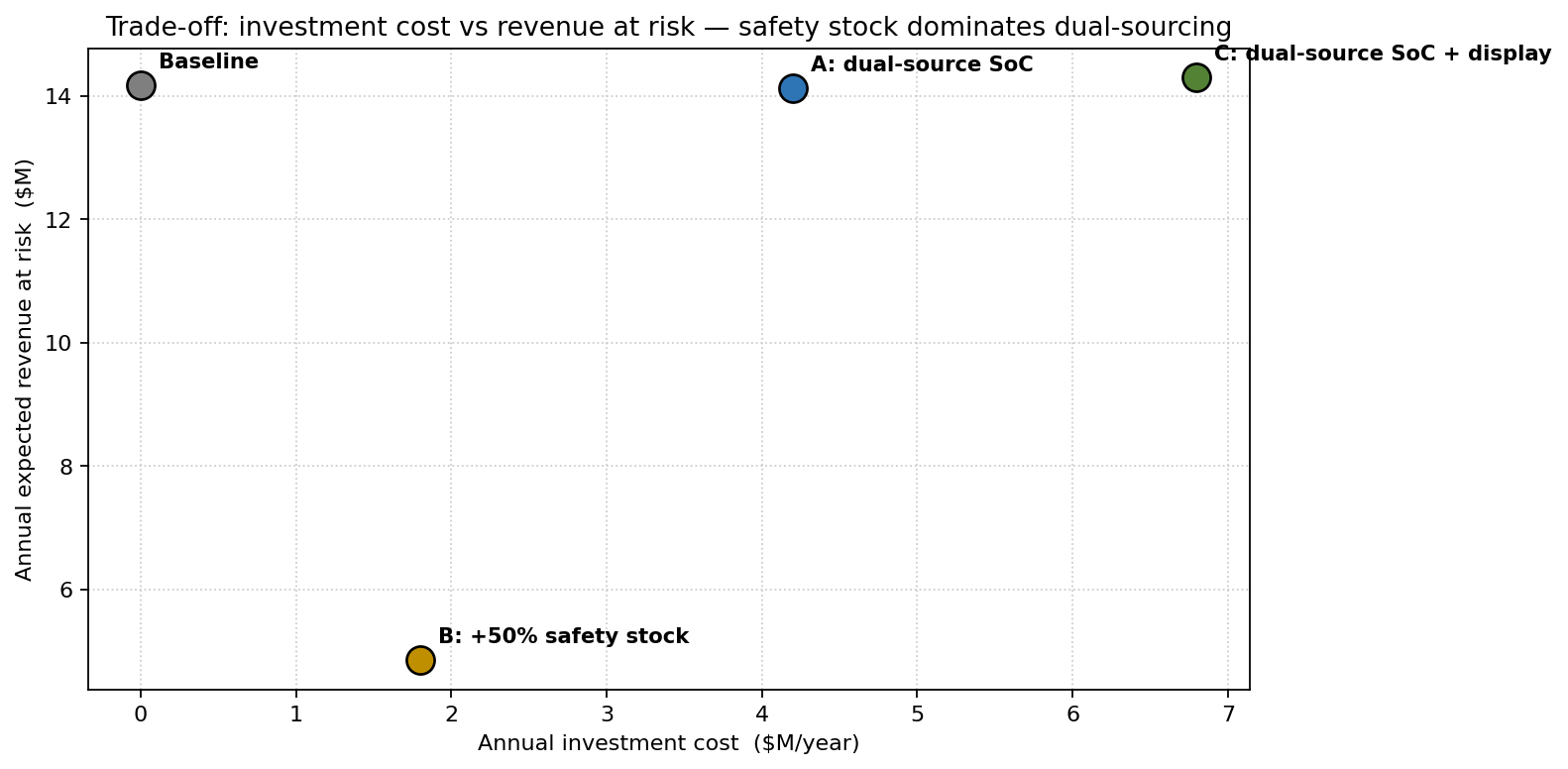
Plotting annualised investment cost against expected revenue at risk puts the four scenarios on the same surface. The dual-source strategies are dominated points — they cost more and leave more revenue at risk than safety-stock expansion. The simulation did not just rank the strategies; it removed two of them from consideration entirely.
From insight to action
- Safety stock expanded across the chain (+50% everywhere), with the biggest absolute weeks-of-cover added on the thinly-buffered binding components the attribution flagged — battery cells (2.0 wk) and PCB assembly (1.8 wk). Total holding-cost increase $1.8M/year, revenue-loss reduction $9.3M/year (from $14.17M to $4.85M).
- Dual-source SoC paused as a primary risk mitigation. The simulation showed it is the wrong instrument for the dominant risk; the resilience case lives on as a longer-horizon strategic option but not as a 12-month spend.
- Display dual-source qualified but not contracted — kept as a stand-by activation option in case the routine LT tail widens (a possibility the simulation flagged as a re-run trigger).
- The simulation became the supplier-review tool: every quarterly supplier scorecard now updates the LogNormal LT parameters from new data and reruns the fill-rate distribution. A widening σ_log on any component now triggers a procurement conversation rather than waiting for the next stockout.
ModelRisk Functionality Used
- LogNormal lead times per component with σ_log calibrated to 18 months of receiving-dock data — the model that exposed the routine tail dominating the disruption tail.
- Bernoulli disruption events with component-specific weekly probability and uniformly distributed extra-week severity — the layer where dual-sourcing matters and which the simulation showed was an order of magnitude smaller than executives believed.
- Weekly-grain inventory simulation with re-order to (LT + safety) × demand target, gating production on the minimum across the five components — captures the multiplicative effect of joint-availability that a per-component analysis cannot.
- Marginal attribution by component and channel — re-running with each component's disruption probability, then its routine lead-time variability, collapsed in turn — gave the per-component dollar contribution that ranked the SoC dual-source case near zero avoided loss and surfaced battery cells and PCB assembly as the true binding constraints.
- Trade-off chart of investment vs revenue-at-risk, with strategy points and Pareto dominance read directly off the plot — the visual that ended the dual-source debate.
The Monte Carlo lesson for supply-chain resilience is that the headline-grabbing risk is not always the dominant risk. Dual-sourcing is the right tool against catastrophic disruption; safety stock is the right tool against routine lead-time tails — and on this chain, the routine tails were roughly 4× larger than the disruptions, and concentrated on the components nobody was watching, a fact only the simulation could show.