

Industry: Manufacturing
Product: ModelRisk
Application: Production Line Optimization
Why the $620k Variability Project Did Not Move the Mean: A Production-Line Stochastic Simulation
A precision-automotive line was missing its 1,100-parts/day delivery commit on roughly one shift in six. Plant leadership had pre-approved a $620k six-sigma project to tighten machining cycle-time variability — the conventional choice and the one the deterministic capacity model endorsed. Before the capex went out, the ops team built a 20,000-day Monte Carlo model in ModelRisk of all four stages — forging, machining, heat-treat, assembly — with cycle times, defects, and reliability events all stochastic. The simulation contradicted the deterministic recommendation: the variability project would lift the P10 by 11 parts/day but the mean by zero, because machining was already running at 97.8% of its dimensional capacity. The money belonged on a fifth machining station, not on a six-sigma kaizen.
The first chart the ops VP saw made the gap unmissable: the deterministic capacity plan promised 1,180 defect-free parts a day, and the simulated distribution sits well below it.
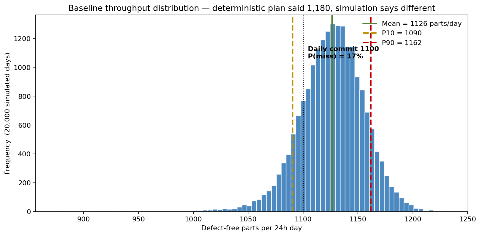
Mean throughput 1,126 parts/day, P10 1,090, P90 1,162, and a 17% probability of missing the 1,100-unit daily commit when a bad MTBF day on machining stacks with a hot defect-rate draw. The deterministic point answer of 1,180 lay outside the P90 — the existing line is closer to its capacity wall than the takt-time spreadsheet had been showing.
A stochastic line, not a takt-time spreadsheet
Each of the four stages has three independent sources of variation:
- Per-part cycle time — LogNormal, because cycle data is right-skewed. Most parts finish near the mode but the occasional slow part has a long tail. Machining median 5.0 min/part with σ_log = 0.30; forging 4.2 min, σ_log = 0.18; heat-treat 4.6 min, σ_log = 0.22; assembly 4.4 min, σ_log = 0.25.
- Defect rate — Beta. Bounded on [0, 1], no Normal-distribution-draws-negative-defect-rate nonsense. Forging and heat-treat run Beta(1.5, 198) ≈ 0.75% mean; machining and assembly Beta(4, 196) ≈ 2.0% mean.
- MTBF and MTTR — failures per 24h drawn from Poisson(24/MTBF) per station, repair time Gamma-distributed with mean = MTTR. Machining: MTBF 1,200 h, MTTR 3.0 h; forging 900/2.5, heat-treat 2,400/4.0, assembly 1,800/2.0.
Each stage runs four parallel stations except heat-treat and assembly which run five. The day's good output for each stage is (parallel_stations × 1,440 min × uptime_fraction / avg_cycle) × (1 − defect_rate). Throughput of the buffer-less line is the minimum of the four stages.
Where the line actually binds
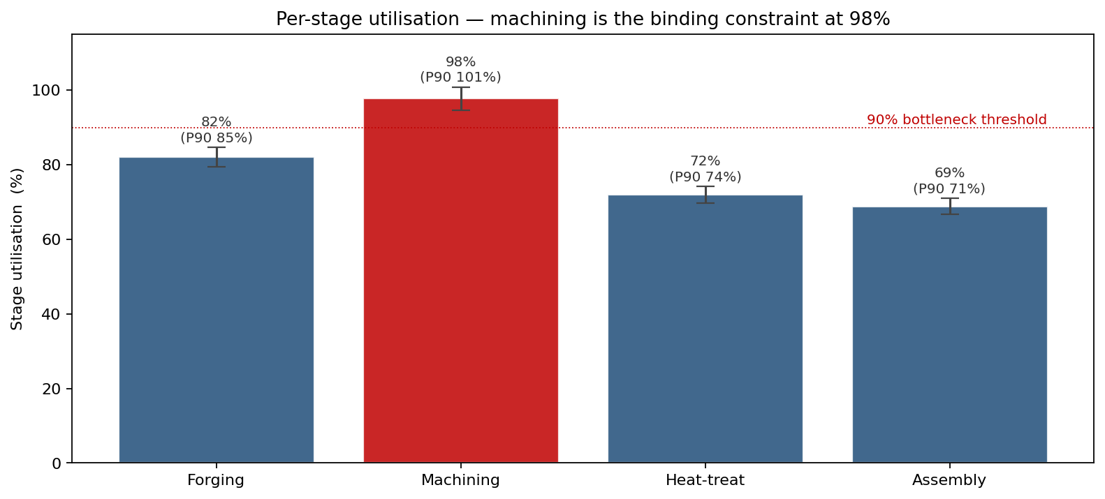
Machining runs at 97.8% utilisation on average with the P90 day hitting 100% capacity — meaning some days the stage cannot keep up with what it ships. Forging at 82%, heat-treat at 72%, assembly at 69% — all have meaningful buffer. This was the picture the team needed before deciding where the $620k should go.
The strategy comparison that changed the decision
Four candidate strategies, all run through the same simulation engine on the same 20,000 days:
- A — machining cycle σ_log 0.30 → 0.18 via operator training and a CAM-program standardisation kaizen. The original $620k plan.
- B — machining MTBF 1,200 h → 2,400 h via predictive-maintenance instrumentation and tool-life tracking.
- C — add a fifth parallel machining station (~$1.1M capex + tooling, longer install).
- D — A + B combined.
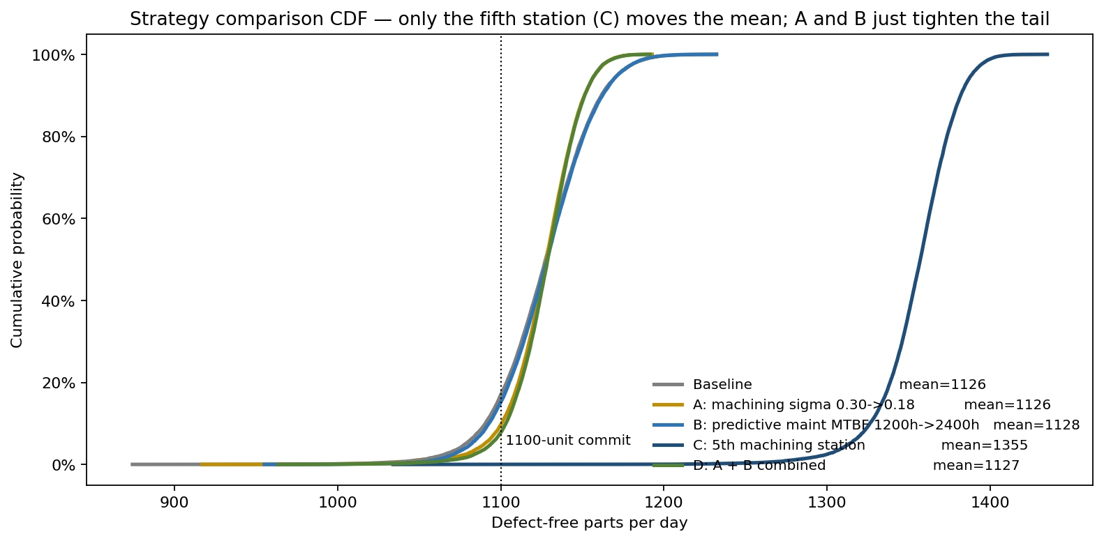
The CDF reveals what the deterministic comparison literally cannot show:
| Strategy | Mean Δ | P10 Δ | Comment |
|---|---|---|---|
| A — variability | +0 | +11 | tightens the tail, no mean lift — machining is already dimensionally capped |
| B — MTBF | +2 | +3 | already-high uptime leaves little room |
| C — fifth station | +229 | +236 | breaks the bottleneck, full mean shift |
| D — A + B | +1 | +13 | both levers wasted while bottleneck holds |
Variability reduction is the wrong intervention on a binding-bottleneck stage. The line gives back the variability gain at the next constraint. This is a finding the deterministic capacity model cannot produce because it has no concept of "binding stage at random across days."
What actually drives day-to-day throughput
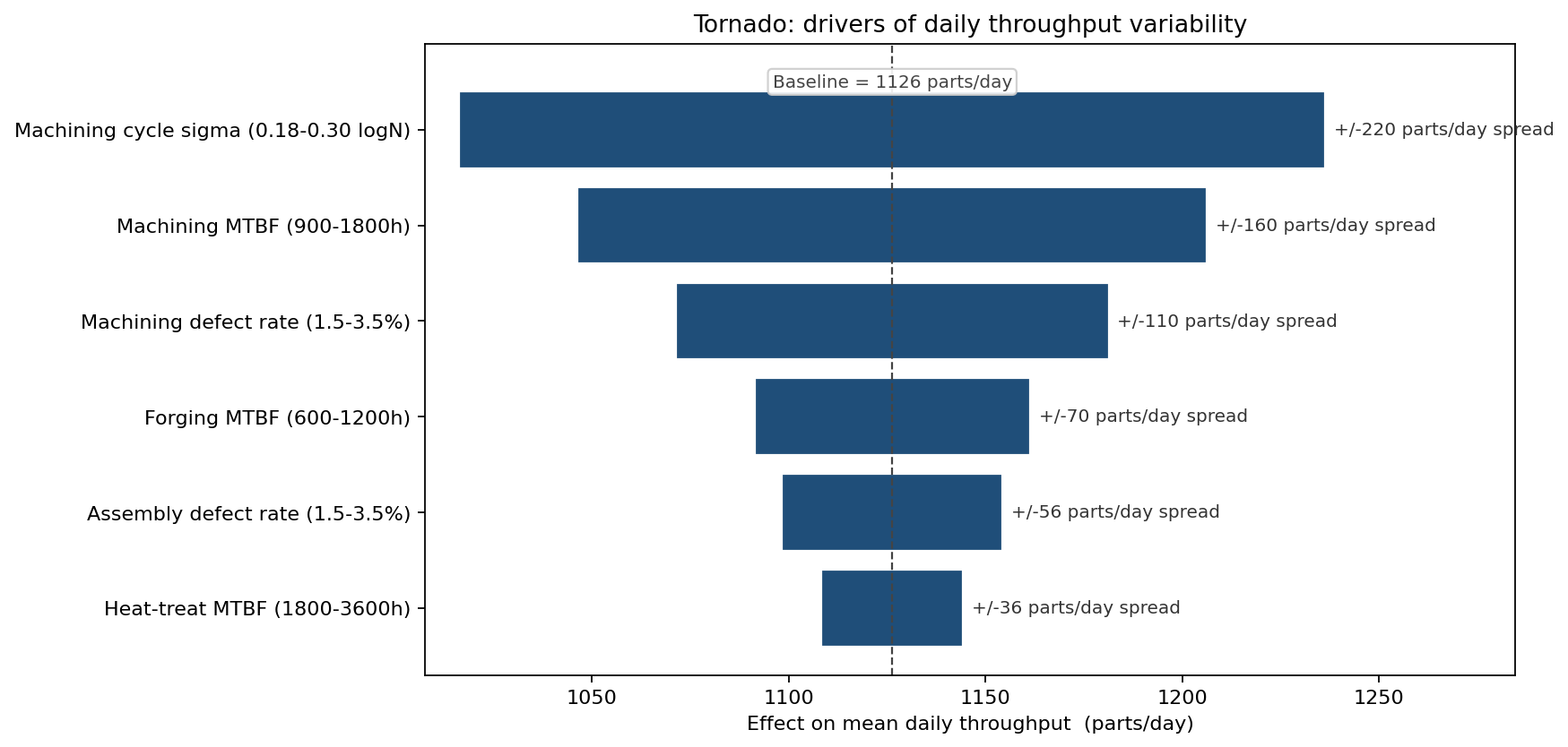
Machining cycle σ_log is still the biggest driver of throughput variance even though it does not move the mean — and that subtlety is the entire point. Variance and mean are different problems with different fixes. The tornado guided the team to budget separately for tail-day risk reduction (variability and reliability levers on machining) and for capacity expansion (fifth station).
From insight to action
- Strategy C approved over Strategy A, even though A was cheaper and had been pre-endorsed. The simulation showed C delivers +229 parts/day mean lift vs A's +0; payback under 11 months at $42 GM per part.
- MTBF instrumentation deferred until the fifth station goes live, at which point machining utilisation drops and the predictive-maintenance investment recovers a meaningful share of its claimed mean lift.
- Daily commit raised from 1,100 to 1,300 parts/day once C lands, with the new P10 at 1,326 supporting the higher promise.
- Capacity model retired; the Monte Carlo workbook is now the line's planning artefact — every shift schedule and customer commit references the simulated CDF.
ModelRisk Functionality Used
- Per-stage LogNormal cycle times with σ_log calibrated to two years of MES data — not the deterministic takt-time line balance the plant had been running on.
- Beta defect rates stage-by-stage, replacing point defect percentages — preserves the bounded [0, 1] property that Normal draws would routinely violate.
- Poisson failures + Gamma MTTR per station instead of a flat OEE multiplier, exposing the bad-MTBF-day tail that drove the 17% miss-commit probability.
- Buffer-less linear-flow throughput aggregation — daily output = min of stage outputs — which is what surfaced machining as a stochastic bottleneck, not just an average one.
- Strategy CDF comparison with mean and P10 deltas explicit, the table that flipped the $620k decision from variability reduction to capacity expansion.
The Monte Carlo lesson for ops engineering is that variability projects and capacity projects are not substitutes. Variability tightens the P10; only capacity moves the mean. Spending variability dollars while the line is at 98% utilisation hides the answer the simulation made unmissable: the fifth station was always the bottleneck.