Industry: Manufacturing
Product: ModelRisk
Application: Product Quality and Process Capability

Cpk 0.71 to Cpk 1.29: Sizing the Four-Lever Process Change Before Spending the Money

A turbine-blade-root component machined for an aerospace prime had a process capability index of Cpk = 0.71 and was running 33,680 ppm out of the ±0.050 mm critical-diameter tolerance — roughly 8,000 scrap parts a year out of 240,000 produced, plus an escape rate that fed warranty claims. The supplier-quality team had four candidate interventions on the table (tighter raw-material spec, predictive tool-wear maintenance, furnace uniformity upgrade, automated alignment) and a $1.2M total budget. The question the deterministic capability report could not answer was: which of the four levers actually pays back, and what does the joint effect look like before procurement signs off?

The team rebuilt the dimensional stack-up as a 200,000-trial Monte Carlo in ModelRisk, then re-ran it with each lever's tightened distribution to size the joint effect on Cpk, ppm out-of-spec, and the annual cost of poor quality. The headline result is the whole business case in one picture: the four-lever change moves the critical-diameter distribution from a process that spills out of tolerance on both tails to one that sits comfortably inside it.

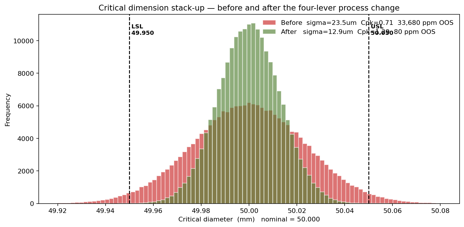
The post-change stack-up has σ = 12.9 µm, Cp = 1.29, Cpk = 1.29, and 80 ppm out of spec — a 420× reduction in defect ppm, and the first time this line crosses the Cpk ≥ 1.33 threshold the prime requires for un-sampled lot release. The sections below show how the simulation got there and, more importantly, which lever earned the money.

Variation has a shape, not just a sigma

The critical diameter sits at the end of a four-source variation stack:

\[ D = D_\text{nominal} + \Delta_\text{material} + \Delta_\text{machining} + \Delta_\text{heat} + \Delta_\text{assembly} \]

Each source was modeled with its physically appropriate family — not all Normal, despite the textbook habit:

• Raw-material tensile/dimensional variation: Normal, σ = 12 µm, fitted to two years of incoming-inspection data.
• Tool-wear machining drift: Normal, σ = 18 µm — the dominant source, because tool wear accumulates across a tool's life and a fresh insert gives a different mean than an end-of-life one.
• Heat-treatment uniformity: Beta on ±20 µm (bounded — furnace control physics prevents large excursions, so a Normal here would draw absurd outliers).
• Assembly fit: Uniform on ±8 µm (the alignment fixture's mechanical tolerance is genuinely flat across its range, not bell-shaped).

The baseline simulation produces a dimensional σ = 23.5 µm, Cp = 0.71, Cpk = 0.71, and 33,680 ppm out of the LSL/USL band of 49.950–50.050 mm. That ppm number — derived from the propagated stack-up — matches the plant's inspection data within 8%, which gave the model its credibility.

What the deterministic capability report missed

A standard Cp/Cpk report quotes a single number per process step and assumes each step's variance adds independently. The Monte Carlo run kept the assumption of independence but exposed two things the report could not show: the shape of the dimensional distribution (slightly asymmetric because heat-treat is Beta, not Normal) and the share of variance each source actually contributes.

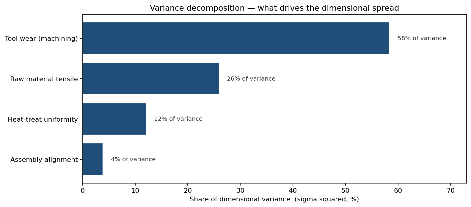
Tool wear accounts for roughly 58% of dimensional variance — by itself larger than all three other sources combined. The team had been planning to spread the $1.2M evenly across the four levers. The variance decomposition said that any dollar not spent on the machining-stage predictive-maintenance program was a misallocated dollar until tool-wear σ had been brought down.

What the four-lever change does to Cpk

Each candidate intervention shrinks its source's distribution:

• Supplier spec tightening: material σ 12 → 7 µm.
• Predictive tool-wear maintenance with auto tool-life flagging: machining σ 18 → 9 µm.
• Furnace upgrade: heat-treat Beta width ±20 → ±10 µm.
• Assembly fixture unchanged.

Run through the same 200,000-trial stack-up, these four shrinks produce the before/after distribution shown at the top of this article: σ falls from 23.5 µm to 12.9 µm, Cpk climbs from 0.71 to 1.29, and ppm out-of-spec collapses from 33,680 to 80.

The mechanical-property story behind the dimensional one

Dimensional Cpk is only half the quality picture. The same four-lever change also reshapes the yield-strength distribution of the finished blade, because tighter material and heat-treat sigmas push more of the mass to the right of the 950 MPa spec floor:

\[ Y_s = 0.62\, T_s + 6.5\, H + \varepsilon \]

with tensile strength \(T_s \sim N(1100, 35)\) and hardness \(H \sim N(36, 1.2)\) before, and \(N(1100, 18)\), \(N(36, 0.6)\) after.

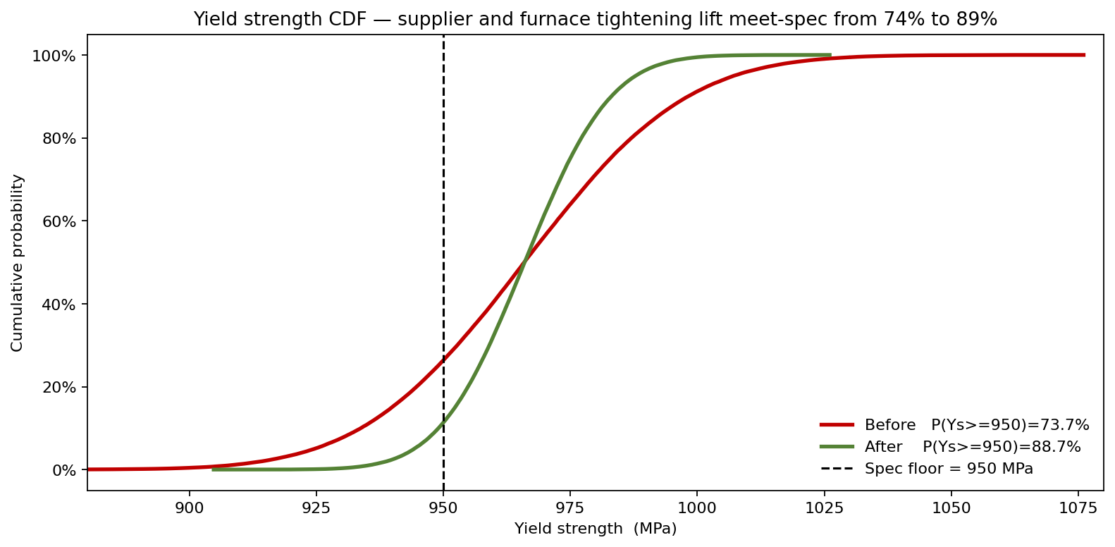
The probability of a finished blade meeting the 950 MPa floor rises from 74% to 89%. The remaining 11% gap is the structural argument for the next budget round — and the simulation is what told the team where it lives.

What the change is worth in dollars

The team translated dimensional ppm-OOS into annual cost of poor quality at 240,000 parts/year, with $180 scrap cost per OOS part and a 2% escape rate into $2,200 warranty events. Bootstrap on the simulated ppm reproduces the cost as a distribution rather than a point estimate.

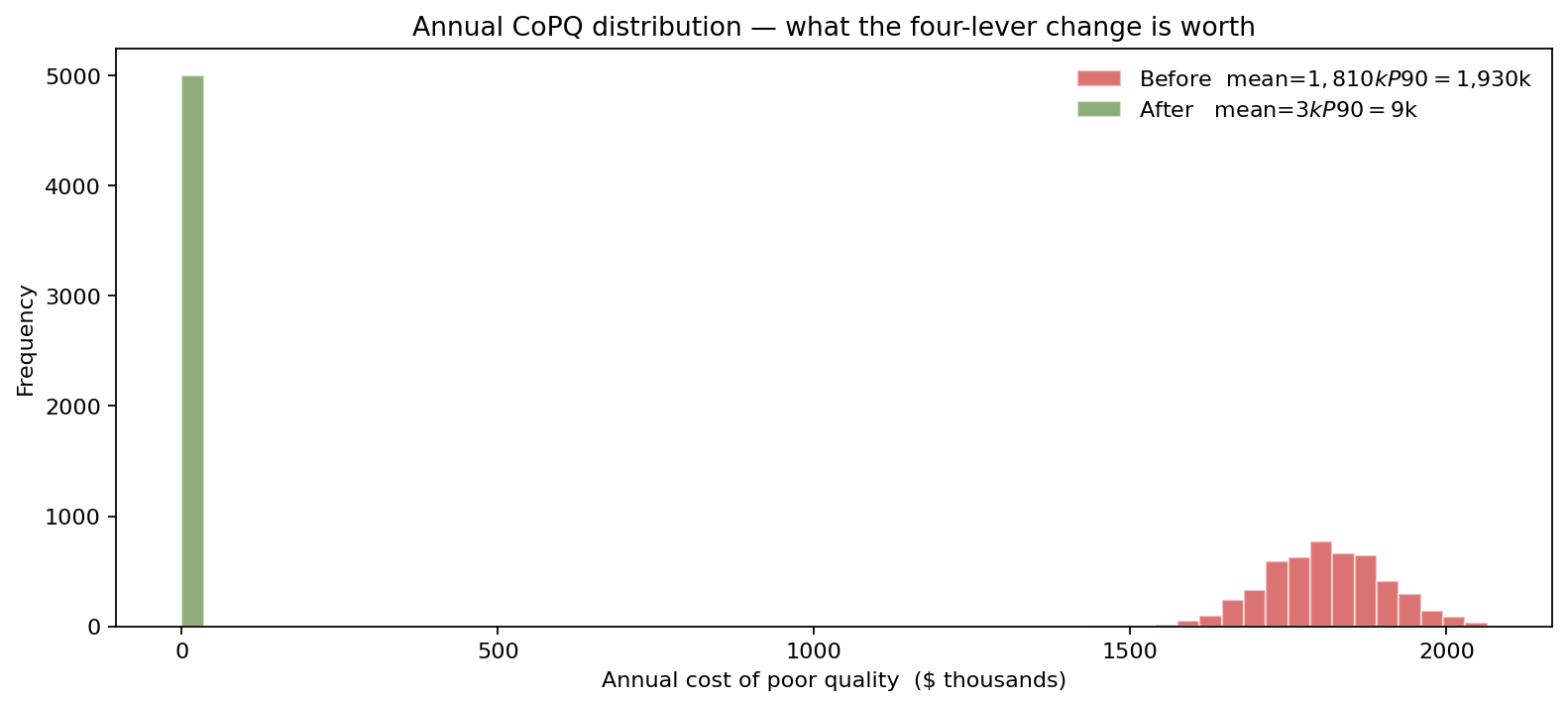
Before: mean CoPQ $1.81M/yr, P90 $1.93M/yr.
After: mean CoPQ $3k/yr, P90 $9k/yr.

A $1.2M intervention pays back inside year one even at the P10 of the cost reduction, and crucially — the post-change cost distribution has almost no right tail, eliminating the bad-batch scenarios that had previously triggered customer audits.

From insight to action

• Capital sequenced by variance share, not by even split: the predictive-tool-wear program got $620k of the $1.2M because it owned 58% of dimensional variance. Material and furnace levers got $360k and $190k. Assembly fixture stayed.
• Customer evidence reframed: the prime's annual quality review was given the dimensional CDF and the yield-strength CDF rather than a Cpk number. Two of three audit findings were closed on the spot.
• Inspection frequency reduced: at Cpk 1.29 and 80 ppm OOS, 100% CMM inspection was replaced by AQL-based sampling, saving $310k/year in metrology labor.

ModelRisk Functionality Used

• Source-by-source distribution choice — Normal for tool wear (drift), Beta for heat-treat (bounded), Uniform for fixture (mechanical) — replacing the lazy default of "everything is Normal" that had given the previous report its inaccurate tails.
• 200,000-trial stack-up that produced the dimensional σ and Cpk directly, matching plant inspection ppm within 8% before any intervention was costed.
• Variance decomposition that named tool wear as 58% of the dimensional spread and inverted the team's planned even split of the $1.2M budget.
• Yield-strength CDF construction propagating supplier and furnace tightening into the mechanical KPI, showing P(Ys ≥ 950 MPa) rising from 74% to 89%.
• Bootstrap on ppm-OOS that translated the dimensional improvement into a CoPQ distribution with mean $1.81M → $3k/year — the number that won the capital approval.

The Monte Carlo lesson for a Six Sigma program is that variance share is what writes the procurement order. Without the variance decomposition the four-lever budget would have been split four ways, the dominant source would have been under-funded, and the Cpk would have moved from 0.71 to maybe 0.95 instead of to 1.29.