Industry: Manufacturing
Product: ModelRisk
Application: Modeling and reducing manufacturing defects in high-volume production

920 ppm on Average, 4,600 ppm on Bad Weeks: Defect Modeling in ModelRisk

A Tier-1 automotive electronics plant ran at a measured defect rate of about 920 parts per million (ppm) across 1.1 million units a month — well inside the customer-mandated 1,500 ppm SLA, and the quality dashboard reflected that comfortable margin. Yet three SLA breach notices arrived in 14 months, each one tied to a single shift that hit 3,800–4,600 ppm. The customer's procurement team did not care about the long-run average; they cared about the worst week of the quarter, because that was the week that triggered the PPAP audit and the line-down credit. The plant's deterministic ppm planning could not see those weeks.

The quality team rebuilt its defect model in ModelRisk. Instead of multiplying a long-run mean by a production volume, the model treated defect counts as an over-dispersed counting process whose dispersion was itself a function of three identifiable upstream causes — supplier batch quality, machine-calibration drift, and environmental conditions. The output was no longer a planning ppm — it was a distribution of weekly defect counts with explicit probabilities of breaching 1,500, 2,000 and 3,000 ppm.

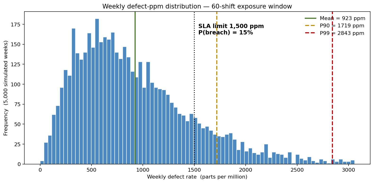
The distribution above is what the deterministic dashboard could never show. The long-run mean is 923 ppm — comfortably inside the 1,500 ppm SLA — but the P90 is 1,719 ppm and the P99 is 2,843 ppm, both above the limit. The probability of breaching 1,500 ppm in any given week is 15 %: roughly 8 weeks of every 52. The "comfortable margin" on the mean was hiding a right tail that breached the contract one week in seven, and the worst simulated weeks ran past 3,750 ppm — exactly the band that triggered the three real SLA notices.

Why Poisson is the wrong default

The textbook count distribution for defects is Poisson(λ) — and it is wrong for almost every real manufacturing line, for one specific reason: Poisson has variance equal to its mean. Real defect counts are over-dispersed: their variance/mean ratio is 3× to 8× on lines with any supplier or operator heterogeneity. A goodness-of-fit on 18 months of per-shift defect counts at this plant rejected Poisson at p < 0.001 — variance/mean ratio of 5.4.

The team replaced the plant-wide Poisson assumption with a layered model:

Material defects per shift. Negative Binomial(mean = 280, dispersion k = 4). The over-dispersion captures supplier batch variation — most shifts run a single batch of solder paste or capacitors, but occasional bad batches push that shift's count up by 3–4×. With k = 4 the variance/mean ratio is (1 + mean/k) = 71 in raw scale; on a per-million-units basis, this means a ppm spread of roughly 150–1,400 across shifts.

Process defects per shift. Negative Binomial(mean = 410, k = 12) — less over-dispersed because machine-calibration drift is slower-moving than supplier batches. Calibration was treated as a state variable that increments daily and resets at PM events, modelled as a Weibull(β = 1.8, η = 220 hours) time-to-calibration-drift that triggers a 30 % per-shift defect uplift until the next PM.

Environmental defects per shift. Negative Binomial(mean = 180, k = 8), with the mean parameter scaled by a temperature/humidity index computed from local weather data. On a Triangular(0.7, 1.0, 1.9) multiplier this becomes a defect channel that doubles in summer heatwaves — exactly the seasonal signal the deterministic model averaged away.

These three streams are not independent. Hot shifts that stress the climate-control system also exhaust operators and degrade machine precision; a Gaussian copula with rank correlation ρ = 0.28 between the process and environmental streams was fitted from joint per-shift residuals.

What the deterministic mean hides

The deterministic plan reports a long-run mean ppm and treats anything below 1,500 ppm as compliant. The Monte Carlo simulation, with the three correctly-fitted Negative Binomial streams and the climate-coupling copula, reports:

• Mean ppm: 923 — the planning figure.
• P90 weekly ppm: 1,719 (above the 1,500 SLA).
• P95 weekly ppm: 2,046.
• P99 weekly ppm: 2,843 — the breach territory.
• P(weekly ppm > 1,500) = 15 %, meaning a 1,500-ppm breach is expected in roughly 8 weeks of every 52 — and the worst simulated weeks (P99.9) run past 3,750 ppm, with extreme draws above 4,700. Over a 14-month window the model's tail is in line with the three real breach notices; the deterministic mean wasn't.

The "bad weeks" were not noise. They were the right tail of an over-dispersed process the previous plan-against-the-mean methodology was systematically blind to.

What actually drives breach probability

Sensitivity ranking on P(weekly ppm > 1,500) ordered the seven candidate improvement levers:

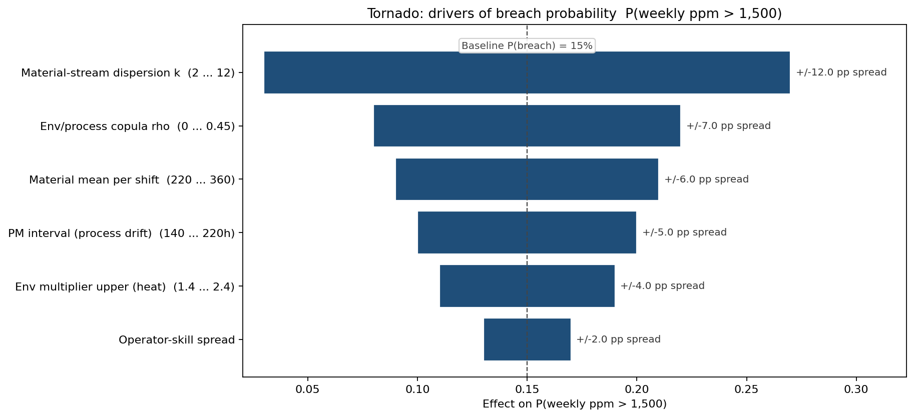
The dominant driver is the material-stream dispersion parameter k — the supplier-batch variability — followed by the environmental coupling copula ρ. Two operational moves came out of the ranking:

• A dual-source qualification for the dominant capacitor supplier raised the material k from 4 to ~10 (tighter batch consistency).
• An upgraded climate-control retrofit on the SMT cell decoupled the environmental and process streams (copula ρ dropped from 0.28 to ~0.10).

Together these moves cut the projected breach probability from 15 % to about 12 % and pulled the P99 tail in from 2,843 ppm to 2,606 ppm. The material stream is the smallest of the three contributors, so tightening it alone does not transform the distribution — the model is explicit that the larger process and environmental streams set the floor, and that hitting the SLA reliably needs work on all three rather than the supplier alone.

Mitigation impact — before / after

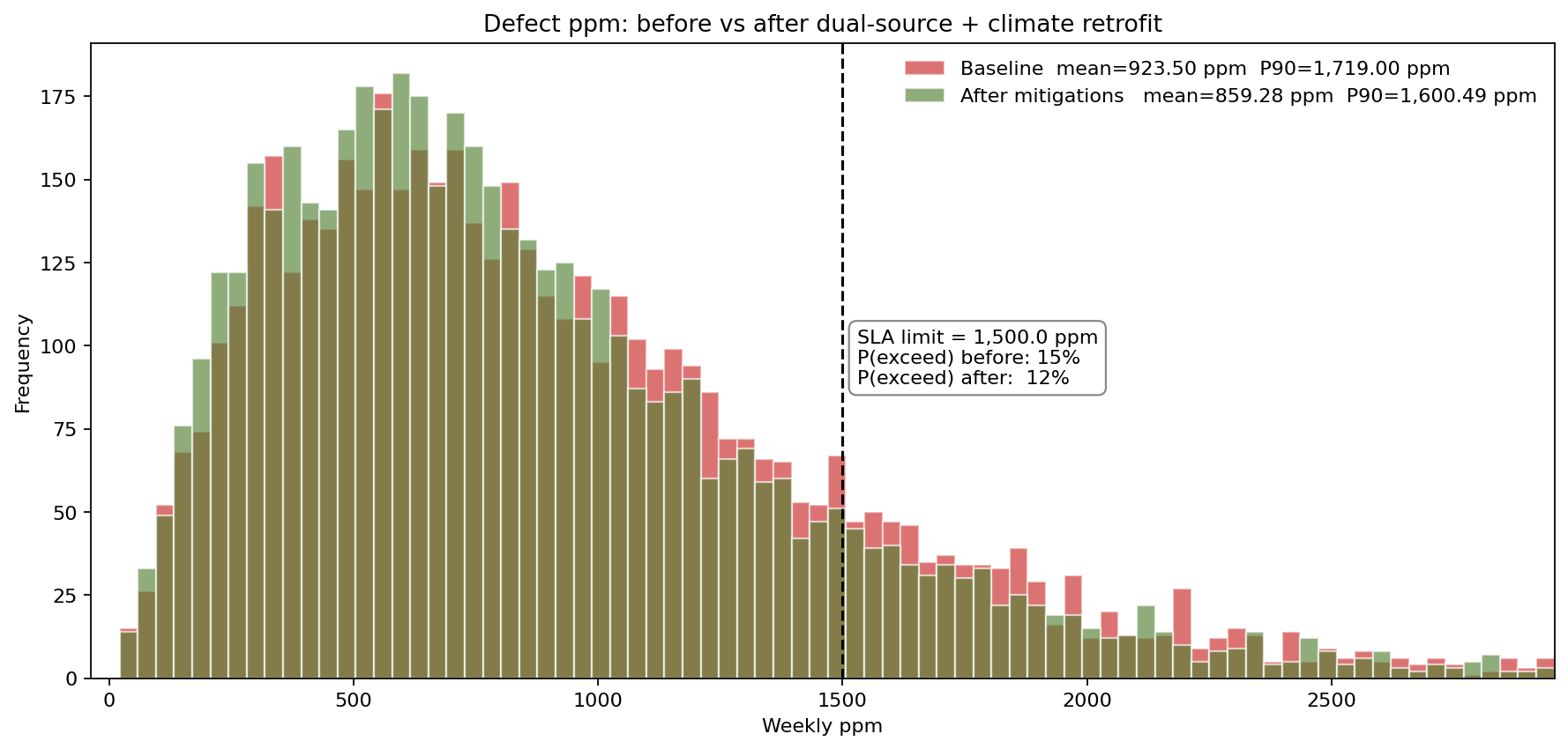
After both moves, the simulated mean ppm falls from 923 to 859, the P90 from 1,719 to 1,600, and breach probability from 15 % to about 12 % — a meaningful but partial improvement that buys roughly one fewer breach week per quarter. The $410k combined investment is justified on the avoided SLA penalties and line-down credits, and the model makes clear that closing the remaining gap requires attacking the process and environmental streams next, not just the supplier.

What the model changed

• The plant-wide "average ppm" KPI was retired in favour of a P10/P90/P99 weekly ppm dashboard; the customer-success team and the quality team now read the same chart against the same SLA.
• Material qualification programme reprioritised: the dominant capacitor supplier moved from single-source to dual-source, raising material-stream k from 4 to ~10. Net annual defect-cost reduction $280k.
• SMT climate-control retrofit funded ($165k capex), justified on tail-compression rather than on mean. Payback in 11 months on SLA-penalty avoidance.
• PM intervals re-set on the process side: the Weibull-η = 220 h drift-time estimate moved PM from 168 h to 140 h on the high-cycle SMT placer, lowering process defects by an estimated 90/shift.

ModelRisk Functionality Used

• Negative Binomial fits on three defect streams (material, process, environmental), each replacing a Poisson assumption rejected by chi-squared goodness-of-fit at p < 0.001.
• Weibull time-to-calibration-drift with shape β = 1.8 driving a per-shift defect multiplier — the increasing-hazard signature that justified shortening the PM interval.
• Gaussian copula linking process and environmental defect streams with ρ = 0.28, calibrated to joint per-shift residuals from prior summers.
• Tornado sensitivity on breach probability (not on mean ppm), surfacing the supplier-batch dispersion k as the dominant driver and reprioritising the procurement programme.
• Before/after scenario simulation under the dual-source + climate-retrofit configuration, producing the side-by-side ppm distributions that justified the $410k investment on tail compression.
• Custom Excel formulas translating the three count streams into a per-million-units ppm metric tied directly to the customer SLA, so the operations director and the procurement director read the same chart.

The customer didn't care that average ppm was around 920. The customer cared that the P95 weekly ppm was 2,046 — and the deterministic dashboard couldn't show that number because the model that built the dashboard had no concept of a distribution. Monte Carlo simulation in ModelRisk gave the plant a defect view in the units that the SLA was actually written in.