Industry: Insurance and Reinsurance
Product: ModelRisk
Application: Risk Pooling

Sizing a Hospital Captive: What 23 Members Really Save by Pooling

Twenty-three regional hospital systems in the United States carry medical-malpractice exposure individually. The largest member pays $28 million a year for primary $5M-limit cover; the smallest pays $1.4 million. A working group has proposed consolidating the layer 0–$5M into a member-owned captive insurer capitalised at $90 million. The question every CFO on the working group is asking is the same: how much does my hospital save by pooling — and what is the probability the captive runs out of capital in any given year?

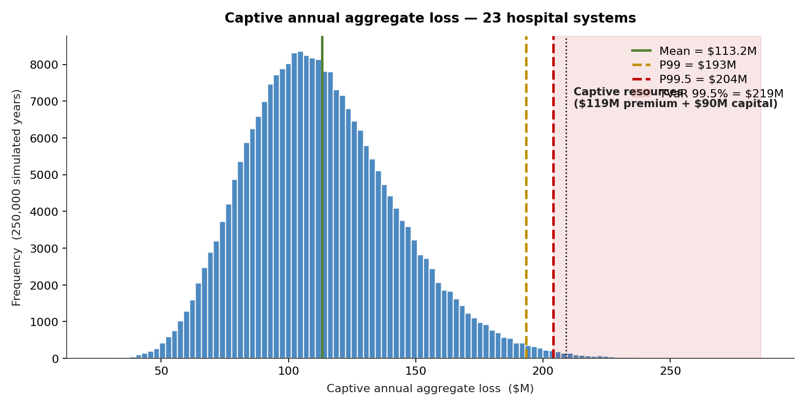
These are not deterministic questions. The savings depend on the diversification benefit between members; the capital adequacy depends on the shape of the aggregate loss distribution, not its mean. A single point estimate cannot answer either. The actuarial team built the captive in ModelRisk and ran 250,000 simulated years. The chart below is the whole case in one picture: the captive's annual aggregate loss, the percentiles that set its capital, and the line marking what year-one resources can absorb.

What pooling actually does to volatility

A pool of \(n\) members reduces volatility if and only if members' losses are less than perfectly correlated. The standard deviation of the pool, expressed as a coefficient of variation, falls roughly as:

\[ \mathrm{CV}_{\text{pool}} \;\approx\; \mathrm{CV}_{\text{indiv}} \cdot \sqrt{\frac{1 + (n-1)\bar{\rho}}{n}} \]

For \(n=23\) members and an average pairwise correlation \(\bar\rho = 0.18\) (estimated from 12 years of joint claims experience plus shared exposure to medical-protocol changes and litigation cycles), the simulation gives a pool CV of 0.26, versus a member-weighted average individual CV of 1.19. That is the entire economic case for the captive, in one number.

But \(\bar\rho\) is itself uncertain. ModelRisk sampled the correlation matrix from a Wishart prior and re-ran the aggregation on each iteration. Across the posterior the pool CV ranges from 0.22 to 0.32 (P10–P90) — the diversification benefit is robust to plausible correlation assumptions but worth quantifying rather than asserting.

Translated into capital, that CV reduction is the whole prize. To self-insure individually to a 1-in-200 standard, the 23 members would collectively have to tie up about $526M of surplus (the sum of each member's own P99.5-minus-mean buffer). Pooled, the captive needs just $91M for the same 1-in-200 confidence — a $436M reduction in capital that no longer has to sit idle on 23 balance sheets. Note that this is almost exactly the $90M the working group proposed to subscribe: the simulation says the captive is sized about right. Pooling does not cut the premium that funds expected losses — that is ~$113M either way — it collapses the capital.

The aggregate loss the captive must finance

Member-level losses were built compound:

• Frequency per member — negative binomial, mean and dispersion fit to each hospital's prior 12 years. The largest member's mean is 18.4 claims per year; the smallest, 1.1. Using Poisson here under-states variance — claims cluster around protocol failures, training gaps, and individual physician issues, so dispersion above 1.0 is the norm in real data.
• Severity per claim — LogNormal body with a Generalised Pareto tail above $500,000. Tail behaviour matters specifically because the captive layer caps at $5M; claims drawn from the tail are the ones the captive pays in full.
• Correlation between members — sampled from the posterior on \(\bar\rho\) as above, applied through a Gaussian copula to the annual severity totals.

The captive's annual loss after the per-claim $5M cap is the distribution shown in the opening chart.

Mean is $113.2M, the 99th percentile is $193M, and the 99.5th percentile is $204M. Premium has to fund the expected loss, so the captive charges about $119M (the $113.2M mean plus a thin expense load); the $90M of member-subscribed capital sits on top as surplus. Together that is $209M of year-one resources, covering 99.6% of simulated years — but the worst 0.5%, the TVaR-99.5 region, still pierces it, which is precisely why a mean-based capital plan is dangerous, as the next section shows.

Why mean-based capital is the wrong starting point

A deterministic actuarial pricing model would compute pool expected losses ($113.2M) and set capital by a rule of thumb — "1.5× expected losses" — giving about $170M of total resources. The simulation rejects that approach. The relevant capital metric is TVaR 99.5%: the average loss in the worst 0.5% of years. That number is $219M, well above the rule-of-thumb resources, and it is what the $119M of premium plus $90M of capital plus member guaranty backing must ultimately clear. Read the mean and you under-fund the captive in exactly the years a guaranty-call lands on members who can least afford it.

Member contribution rules — fair vs simple

The hardest governance question in a pool is not "what does it cost?" but "what does each member owe?" Two contribution formulas were tested in simulation:

• Stand-alone pricing — each member pays what the pool's actuary would charge them individually. Simple to communicate. But it ignores diversification: small members pay disproportionately for variance they help the pool absorb.
• Marginal capital contribution — each member's premium plus capital charge equals their marginal contribution to TVaR 99.5%. Fair in the actuarial sense (no member is worse off in the pool than alone), but requires re-running the simulation when membership changes.

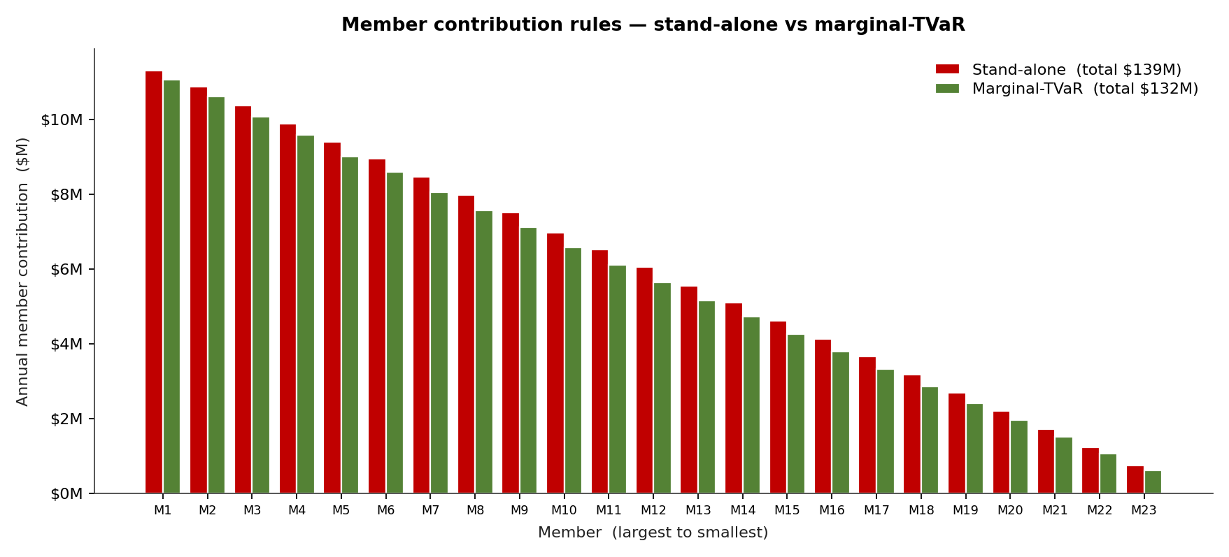
Under stand-alone the four smallest members overpay by 12–21% relative to their marginal-TVaR contribution; switching to marginal-TVaR leaves the largest member essentially flat (down about 2%) while every member is provably no worse than going alone. The working group chose marginal-TVaR for capital allocation and stand-alone for premium, with a five-year re-base. ModelRisk's per-iteration access to the marginal contributions made the calculation auditable rather than a black box.

Where the captive is most exposed

A tornado on the captive's P99 aggregate loss ranks the parameters that move tail capital.

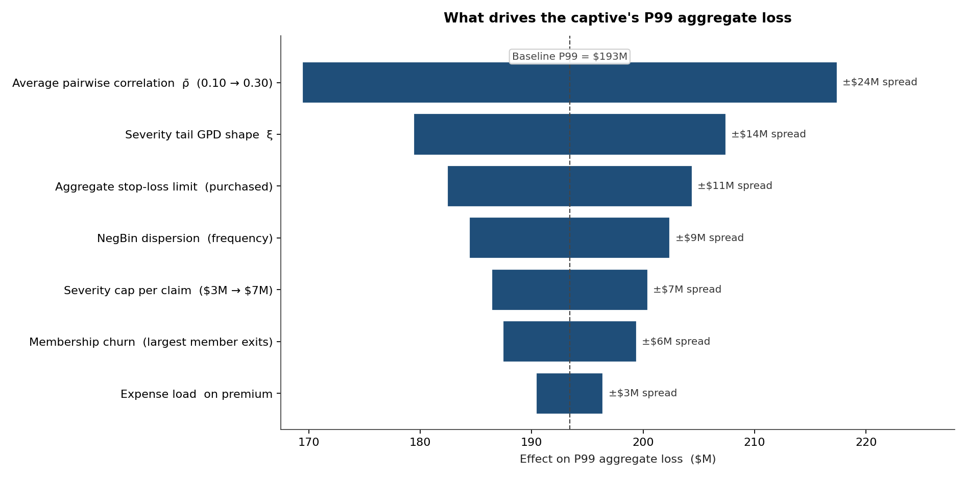
The top driver — by a wide margin — is the average pairwise correlation \(\bar\rho\). A drift in \(\bar\rho\) from 0.18 to 0.30 (plausible if a single tort-reform reversal hit several states at once) raises the captive's P99 by $24M. The captive's reinsurance structure (a $50M xs $50M annual aggregate stop-loss) and the tail GPD shape parameter rank next. The working group used the tornado to define three monitoring triggers: any reading above 0.25 on the running 3-year correlation estimate, any state-level tort-law change in a member's geography, and any aggregate-stop-loss capacity issue at renewal each trigger a special re-pricing review.

Three governance and reinsurance configurations

To make the capital plan defensible, three configurations were compared.

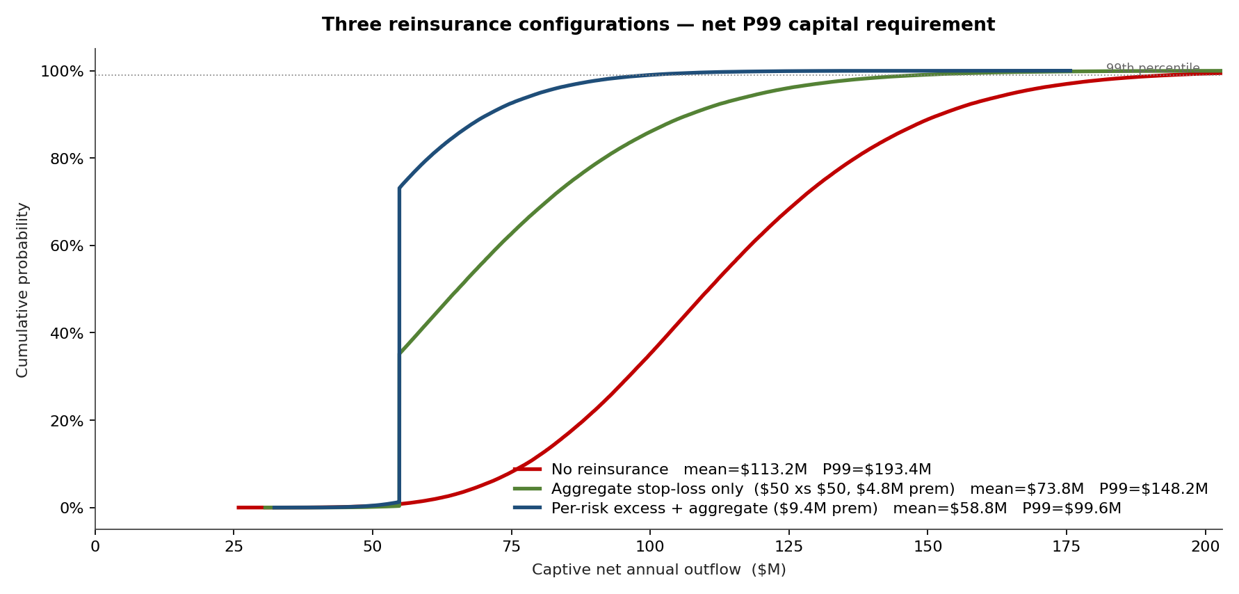
• No reinsurance — captive bears the full layer. P99 net outflow $193M.
• Aggregate stop-loss only — $50M xs $50M annual aggregate. P99 falls to $148M. Cost: $4.8M premium.
• Per-risk excess — $3M xs $2M per claim plus the aggregate stop-loss. P99 falls to $100M but premium rises to $9.4M; the extra capital relief costs more than its capital cost at the captive's cost-of-capital target.

The pool chose the aggregate stop-loss alone, freeing $45M of P99 capital that members otherwise would have had to subscribe.

What changed for the members

• Capital tied up across the 23 members fell from a combined ~$526M to a single $90M captive surplus — a ~$436M release of idle balance-sheet capital, the true diversification dividend. The premium that funds expected losses (~$113M) was essentially unchanged; pooling collapsed the capital, not the premium.
• Capital subscription per member is, for every member, lower than the regulatory capital they would carry stand-alone, and the marginal-TVaR formula makes that demonstrable on demand.
• Three members previously buying only $3M limits could afford the full $5M layer inside the pool — a coverage upgrade that did not exist in the stand-alone world.
• The governance document specifies the simulation as the binding pricing reference, re-run quarterly with member exposures refreshed and the correlation posterior updated for new claims.

ModelRisk functionality used

• Per-member compound frequency-severity simulation with negative binomial frequencies fit individually to each hospital's 12-year history via VoseFitDistribution.
• Gaussian copula on annual severity totals with the correlation matrix itself sampled from a Wishart prior — captures the uncertainty in \(\bar\rho\), not just its central value.
• Marginal-TVaR contributions computed in-simulation by tagging each iteration's tail outcomes and attributing them to member contributions — became the captive's capital allocation rule.
• Aggregate stop-loss and per-risk excess mechanics evaluated as custom Excel formulas per simulated year, with reinstatement accounting and premium-as-percentage-of-limit handling built in.
• Tornado output ranking \(\bar\rho\), tail GPD shape, and reinsurance limit as the three actionable monitoring triggers — informed the captive's governance manual directly.

The mathematics of pooling is old; the captives that fail are the ones whose capital plan was built on a mean and whose contribution rule was built on simplicity rather than fairness. Monte Carlo simulation lets a working group sit down with a distribution of possible bad years and design the governance and reinsurance structure that survives them — which, in the end, is what a captive is for.