Industry: Insurance and Reinsurance
Product: ModelRisk
Application: Catastrophe Modeling

Pricing the 1-in-200-Year Hurricane

A single Category 5 hurricane making landfall in Florida can move a P&C insurer's combined ratio by 20 points in 48 hours. Yet the standard vendor catastrophe models — the ones every reinsurer benchmarks against — hand back a small set of point estimates and a black-box methodology. For an insurer pricing reinsurance, allocating capital under Solvency II, or stress-testing a portfolio against climate scenarios, point estimates are not enough. The risk lives in the tail, and the tail is exactly what a deterministic answer cannot show.

A property and casualty group with $20 billion of insured value across U.S. coastal exposures rebuilt its catastrophe view from the ground up in ModelRisk. The goal: a transparent, fully probabilistic model that produced not one PML number, but a full exceedance-probability curve — the slope of loss against return period that underwriters and rating agencies actually read:

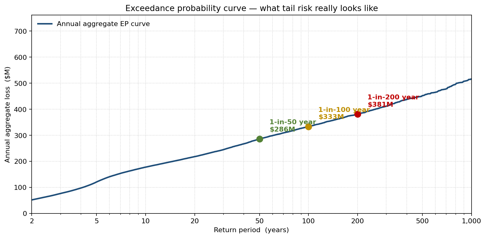
A deterministic spreadsheet has a single point on this curve; the simulation has the whole thing. The 1-in-50 year costs $286M, the 1-in-100 year $333M, the 1-in-200 year $381M — and the slope between them is what prices reinsurance. Below is how the team built it, open and auditable inside Excel.

The three layers of a cat model

Catastrophe modeling stacks three uncertainties: how often events happen, how severe each one is, and how badly the insured assets are damaged. Each layer needs its own probabilistic treatment.

Hazard frequency. The number of land-falling Atlantic hurricanes in a given year was modeled as Poisson with rate \(\lambda = 4\), calibrated to the 1900–2024 HURDAT2 record adjusted for recent decadal warming.

\[ P(N = k) = \frac{\lambda^k e^{-\lambda}}{k!} \]

Storm severity. The body of the severity distribution (industry-level ground-up loss per storm) was fitted as LogNormal, but the model swaps to a Generalized Pareto tail above the $20B industry-loss threshold. This is the standard peaks-over-threshold (POT) construction in extreme value theory — a single LogNormal or Weibull undersells the right tail, where the catastrophic events live.

Vulnerability. Damage ratio (proportion of asset value destroyed) given hazard intensity was modeled by construction class and occupancy with Beta distributions, calibrated to claims data from prior land-falls. Beta is bounded on [0, 1], which a damage ratio also must be — using Normal here, as many in-house models do, lets the simulator draw negative damage or damage above 100%.

Financial loss. For each simulated event the insurer's loss was:

\[ \text{Loss} = \min\bigl(\max(DR \times EV - D, 0),\; L\bigr) \]

where \(DR\) is the damage ratio, \(EV\) the exposure value, \(D\) the deductible, \(L\) the policy limit. ModelRisk evaluates this inside Excel against the live exposure schedule, so changing the schedule and re-running takes minutes, not days.

What the deterministic view misses

A traditional spreadsheet built on historical averages reports the annual average loss (AAL) = $75.5 million. From AAL alone, capital looks comfortable. The simulation tells a different story.

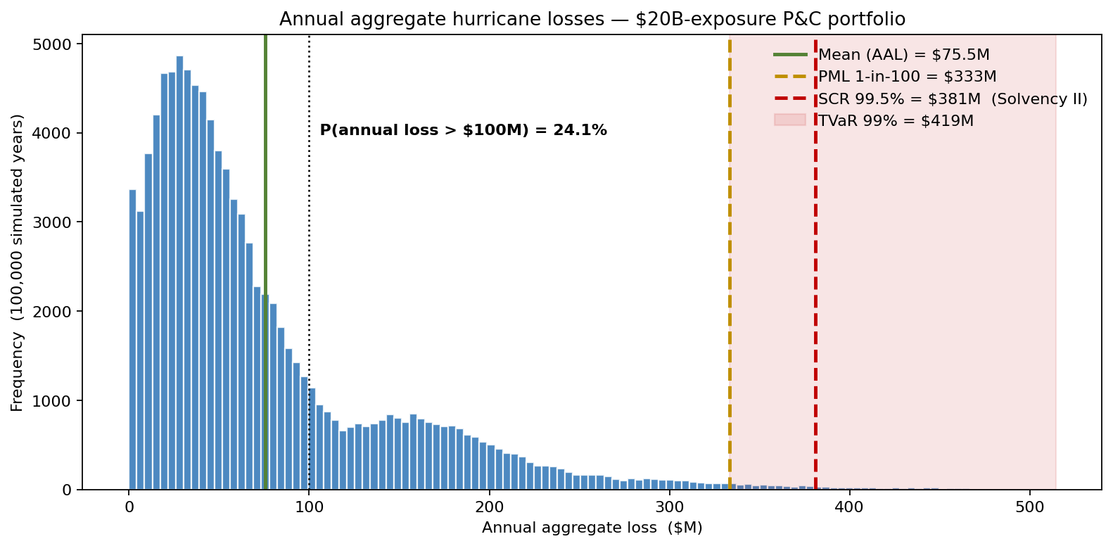
The same portfolio has a 1-in-100 PML of $333 million — more than four times the AAL. The 99.5th percentile, which Solvency II uses to set the Solvency Capital Requirement, is $381 million. And conditional on a tail event, the average loss is $419 million (TVaR 99%). Roughly 24% of simulated years see aggregate losses above $100M. A capital plan built on the mean is built on the wrong number.

The same data plotted on a return-period scale is the exceedance-probability curve shown at the top of this article. The slope of that EP curve in the 1-in-50 to 1-in-200 range is what determines reinsurance pricing — and it's a slope the deterministic model literally does not have.

What actually drives the PML

Sensitivity analysis ranks where the 1-in-100 PML uncertainty lives.

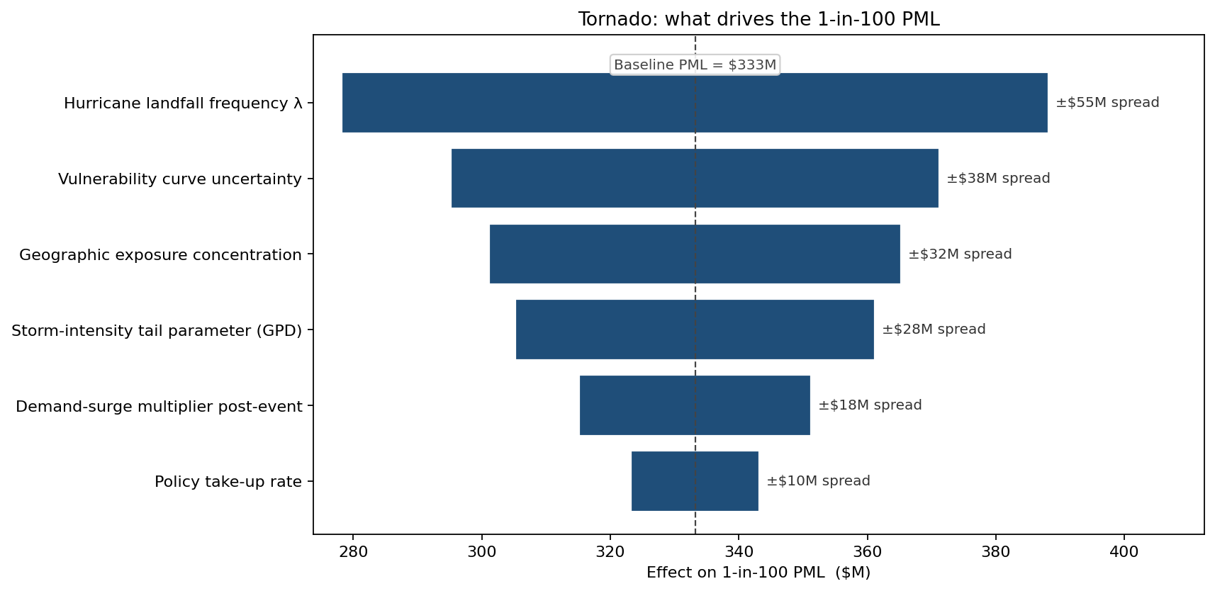
The ranking is itself a research agenda. The biggest single mover is hurricane landfall frequency \(\lambda\) — a parameter pulled from a 124-year climate record that recent science says is changing. Investing in better Atlantic-basin frequency estimates is the highest-marginal-value data project for this portfolio. Vulnerability-curve uncertainty ranks second, which directs the next dollar of investment to claims-data mining from prior events. Reading the chart left to right, the actuarial team had its prioritized work plan for the year.

Optimizing the reinsurance tower

The most consequential application was reinsurance purchasing. Each candidate tower (attachment, limit, premium, reinstatement terms) was run through the same simulation. Comparing two excess-of-loss treaties — the current $50M attach / $200M limit at $12.0M premium against a higher-retention $75M attach / $200M limit at $9.6M premium — produced this comparison of total annual cost (retained loss + premium):

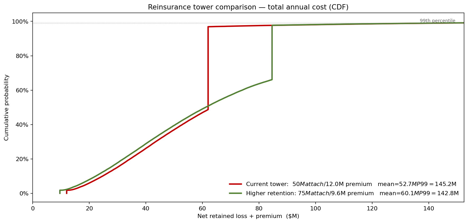
Mean total cost rises by $7.4M when raising the attachment — the insurer retains the $50M–$75M band that the lower attachment had ceded — but the 99th-percentile total cost actually drops by $2.4M, because the same $200M limit attaching at $75M now extends cover to $275M instead of $250M, catching more of the extreme tail. For an insurer judged on capital efficiency, the higher-retention option is better in the tail, slightly worse on average — exactly the kind of trade-off the deterministic comparison cannot frame.

Regulatory capital and rating agency dialogue

Solvency II requires capital to cover the 99.5th-percentile annual loss. The same simulation that produced the EP curve produced SCR contribution by line of business and by geography, allowing the capital team to allocate fairly and to back up the numbers under regulator questioning. Rating agencies — A.M. Best, S&P — increasingly require Own Risk and Solvency Assessment (ORSA) submissions to show explicit probabilistic tail metrics, not just sensitivities. ModelRisk's output formats slotted directly into both workflows.

What changed

• Reinsurance spend down ~15% at constant tail protection, driven by repricing the existing tower against a transparent in-house view of EP rather than vendor-supplied PML points.
• SCR allocation improved: high-PML Gulf states were correctly assigned a larger share of capital, freeing up capital from previously over-charged Northeast portfolios.
• Pricing repaired in two states where premium rates were demonstrably insufficient versus simulated expected loss — a finding the deterministic model had hidden.
• A working model the actuaries own. The vendor cat model is still consulted as a benchmark, but the in-house ModelRisk version is what underwrites, what reports to capital committee, and what the regulator sees.

ModelRisk Functionality Used

• Monte Carlo simulation across the full year: Poisson event count → severity draw → vulnerability draw → financial loss, aggregated across the portfolio over 100,000 simulated years.
• Peaks-over-threshold construction: LogNormal severity body with a Generalized Pareto tail above the $20B industry-loss threshold, calibrated to historical extreme events.
• Beta vulnerability fits to claims data by construction class and occupancy, with the fitting dialog used as the iteration interface for actuarial reviewers.
• Custom Excel formulas for the deductible-and-limit loss function and for portfolio aggregation across policies and treaties — no scripting required.
• Sensitivity ranking that produced the ordered driver list above, used to prioritize the year's data and research investments.
• Exceedance probability and TVaR outputs in the format Solvency II QRT submissions and rating-agency ORSA filings expect.

Catastrophe risk is not the average. It is the shape of the right tail, the slope of the EP curve, and the conditional severity above the threshold. Monte Carlo simulation in ModelRisk is what makes that shape visible — and once it is visible, every downstream decision — reinsurance, capital, pricing, regulatory dialogue — can be made on what the portfolio actually risks rather than on what it averages.