Industry: Healthcare and Epidemiology
Product: ModelRisk
Application: Emergency room optimization

Door-to-Doc Under M/G/c Queueing: Where a Metropolitan ED Loses Its 2% LWBS Target

The Centers for Medicare and Medicaid Services benchmark "left without being seen" (LWBS) at roughly 2% of all emergency department visits. The national average sits closer to 2.6% and individual urban EDs running near capacity routinely log 4–8%. Every LWBS patient is a recovered safety incident at best and a malpractice claim at worst — and almost every LWBS event is a consequence of one thing: the wait-time distribution's upper tail exceeds the patient's tolerance to stay. The mean wait of 40 minutes says nothing about that tail; the histogram below does, and it is where the LWBS exposure actually lives.

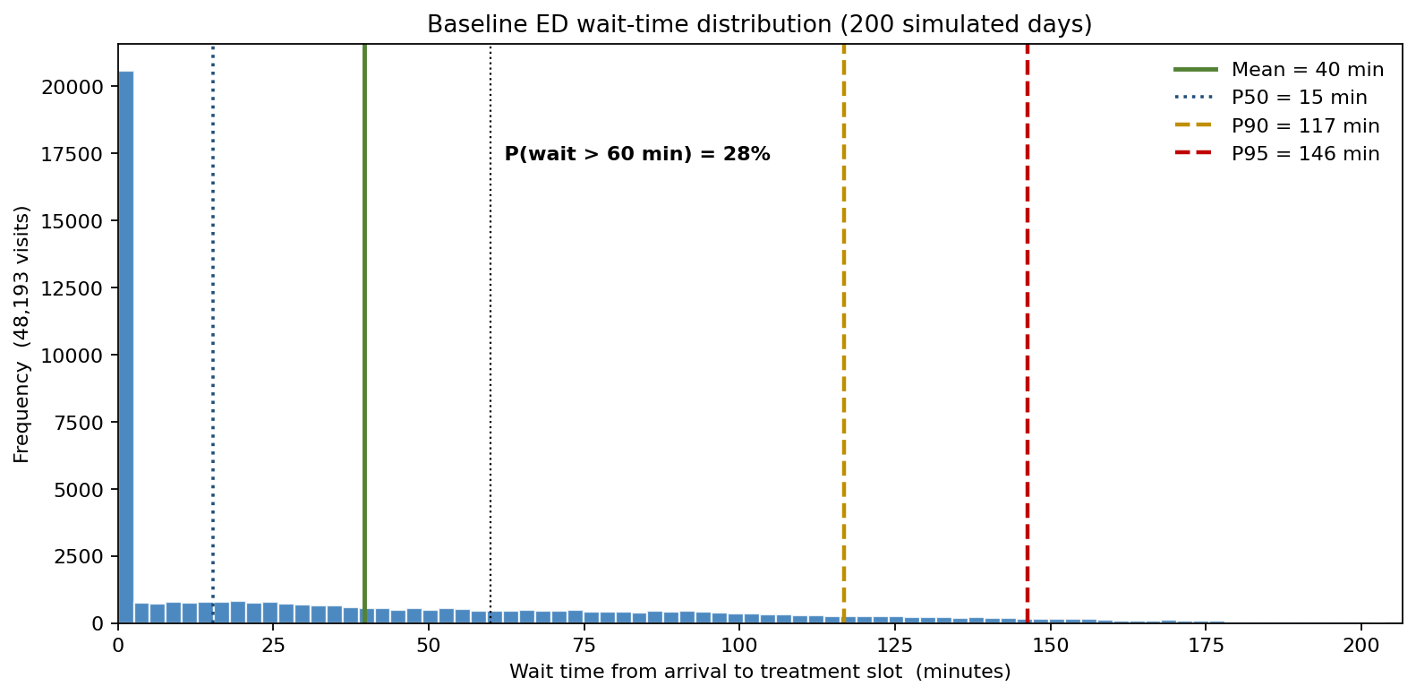
A 240-visits-per-day metropolitan ED in the United States rebuilt its operations model in ModelRisk using an M/G/c queueing structure with non-homogeneous Poisson arrivals and lognormal service times. The deterministic plan, sized to mean throughput across 23 treatment slots, reported a comfortable 40-minute mean wait. The simulation showed the P90 wait at 117 minutes, an LWBS rate of 7.5%, and named two interventions that bring both numbers inside benchmark.

Why M/G/c is the right shape, not a single-server queue

Arrivals. ED arrivals are well-modeled as a Poisson process when sliced into hourly windows, but the rate is not constant: it follows a strong diurnal pattern, with overnight rates around 4–5 arrivals per hour climbing to a 16-per-hour midday-evening plateau. ModelRisk implemented a non-homogeneous Poisson process with piecewise-constant hourly λ — this is the M in M/G/c, but appropriately time-varying.

Service time. Total ED visit duration (triage through disposition) is heavily right-skewed: most visits clear in under 90 minutes, a long tail of complex workups runs past 6 hours. The lognormal distribution — median 95 minutes, σ_log = 0.55, with an acuity multiplier of 1.6× for ESI 1–2, 1.1× for ESI 3, and 0.6× for ESI 4–5 — captures the skew correctly. This is the G (general service) in M/G/c. Using exponential service times, which a textbook M/M/c uses, materially understates the tail and so underestimates the LWBS rate.

Slots (c). Twenty-three concurrent treatment slots represent rooms × physician coverage — the number that keeps a 240-visit-per-day ED with these service times below saturation at the midday peak. This is the c in M/G/c. The scenarios manipulate c.

LWBS trigger. Every 30 minutes a patient has been waiting beyond a 90-minute tolerance threshold, they leave with probability 0.40. This is a separate Bernoulli draw per patient — the correct combination of a probability with a wait-time random variable, not a deterministic threshold.

Baseline wait — where the 95th percentile actually lives

The mean wait of 40 minutes hides everything. P50 is 15 minutes — half of patients are seen quickly. P90 is 117 minutes and P95 is 146 minutes — the upper tail is where LWBS lives and where the patient-safety risk concentrates. The probability that any given visit waits more than 60 minutes is 28% under baseline. Capacity planning to the mean and reporting P95 to the medical executive committee are two different management activities.

Four staffing scenarios, four wait CDFs

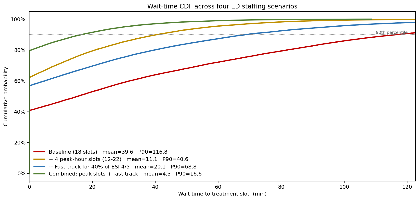
Each curve is one operating model.

• Baseline (23 slots, no fast track): P90 wait 117 minutes, LWBS 7.5%.
• + 4 peak-hour slots (12:00–22:00): P90 falls to 41 minutes, LWBS to 0.2%. Cost: an additional 40 physician-hours per day.
• + Fast-track for 40% of ESI 4/5 patients (low-acuity patients diverted to dedicated nurse-practitioner cubicles): P90 to 69 minutes, LWBS to 2.0%, at lower marginal cost than adding peak slots because NPs cost less than physicians.
• Combined (peak slots + fast track): P90 falls to 17 minutes, LWBS to near 0% — below the CMS benchmark with wide margin.

The LWBS comparison, on one chart

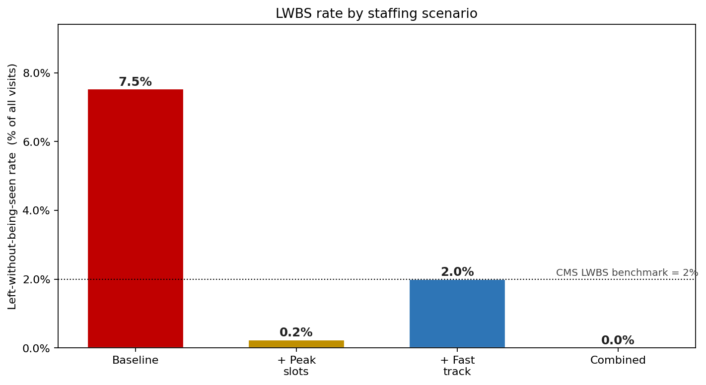
Either single intervention brings LWBS to benchmark in isolation — the fast-track option lands right at the 2% line, the peak-slot option well below it — and the combined intervention drives it to near zero. The ED leadership picked the combined option because the headroom matters: a near-zero baseline LWBS leaves room for an unscheduled physician absence to push the day to a couple of percent and still hold benchmark, where a fast-track-only configuration sitting at 2% would breach on the same off-day.

What actually drives the tail

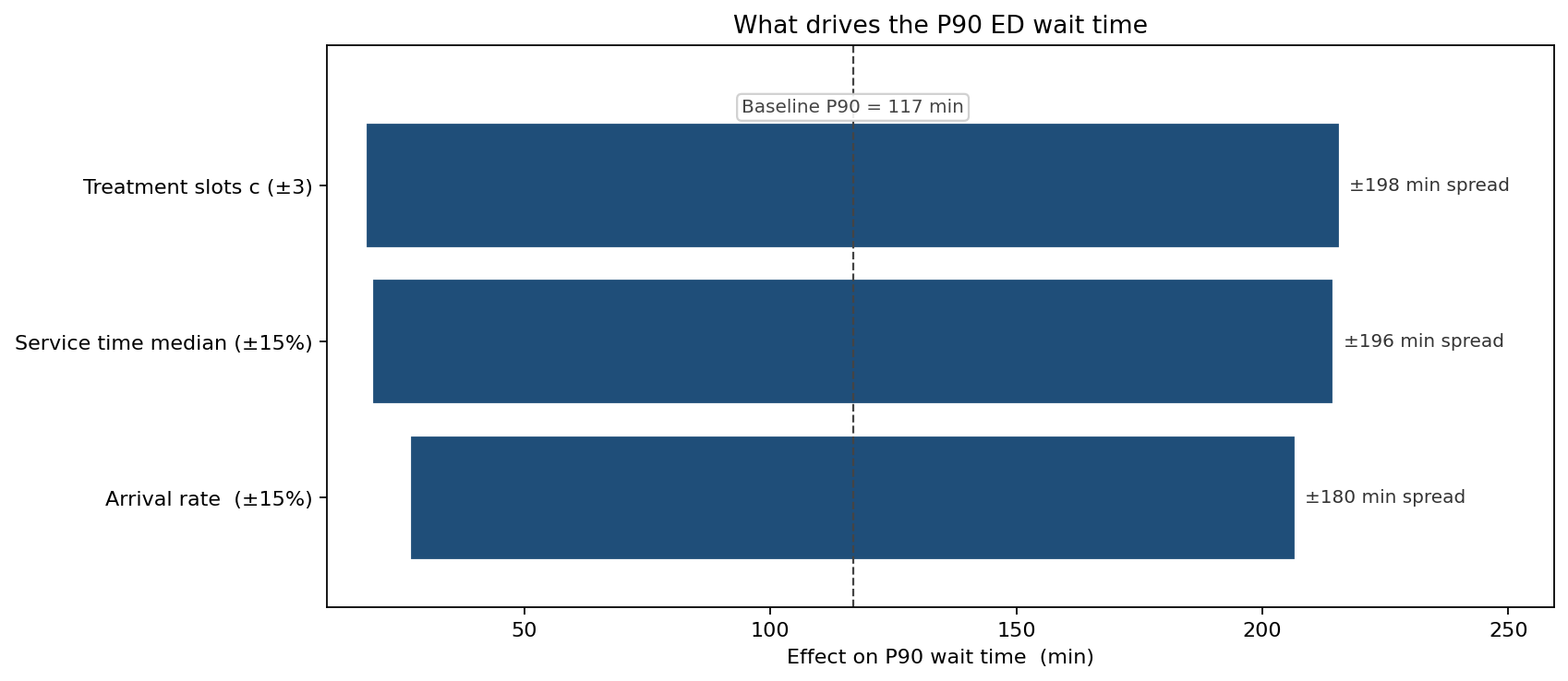
Near capacity, the three levers are roughly co-equal: a 15% arrival-rate change, a 15% service-time-median change, and a ±3-slot change each move the P90 wait by about 90–100 minutes. That co-equality is itself the finding — when an ED runs close to the saturation knee, a single bad-flu-week 15% arrival surge is as damaging as losing three treatment slots, and it is the one input the ED does not control. The ED's first-line response to seasonal surge is therefore not to "absorb at the margin" but to pre-call surge staffing as soon as the daily arrival rate runs above expected, because arrival rate is the leading indicator and wait time is the lagging one.

What changed

• Combined intervention adopted — peak-hour slots + fast track — with the simulation backing the cost case to the hospital finance committee.
• LWBS reporting upgraded from monthly mean to daily P90-wait and rolling 7-day LWBS — the metrics the simulator showed matter for safety.
• Surge protocol triggered on arrival rate, not on wait time — the tornado made the case that arrival rate is the leading indicator and wait time is the lagging one.
• Service-time process improvement targeted at ESI 3 — the largest acuity bucket and the one whose service-time median moves the P90 most.

ModelRisk functionality used

• Non-homogeneous Poisson arrivals with a diurnal pattern scaled so the 24-hour integral is ~240 visits/day (a roughly 14/hr midday plateau falling to ~4/hr overnight), implemented as piecewise hourly λ — the correct generalization of M/M/c arrivals to a real ED.
• LogNormal service times (median 95 min, σ_log = 0.55) with acuity multipliers per ESI tier — captures the right tail that exponential service times miss.
• Discrete-event slot scheduler simulating 23 main + 4 peak-hour slots + 4 fast-track slots, with the door-to-doc clock starting at arrival and stopping at slot assignment.
• Probabilistic LWBS trigger — Bernoulli draw every 30 minutes past the 90-minute tolerance threshold, the correct way to combine a probability with a waiting-time RV.
• 200-day simulation producing roughly 48,000 visit-level outcomes per scenario, enough to estimate the upper-tail percentiles reliably.
• Tornado driver ranking that showed arrival rate, service-time median, and slot count to be co-equal levers near capacity — and singled out the uncontrollable one, arrival surge, to inform the surge-protocol trigger redesign.

The mean wait time is a vanity metric in emergency medicine. The patient-safety and CMS benchmark numbers live in the P90 of the wait distribution and in the LWBS tail — and only a stochastic queueing simulation can size capacity to those numbers rather than to the mean.