Industry: Government and Public Sector
Product: ModelRisk
Application: Policy evaluation

The Headline Said the Minimum-Wage Reform Lifted Youth Employment by 1.1 Points — There Is a 13% Chance It Did the Opposite

Two years after a minimum-wage increase took effect in a set of treated regions, the evaluation unit produced the number the ministry had been waiting for. A difference-in-differences (DiD) study estimated the reform's effect on the youth employment rate at +1.10 percentage points, with a regression standard error of 0.55 pp. The press release wrote itself: the policy worked, and it nearly delivered the +1.5 pp that ministers had promised when they tabled it.

But a DiD point estimate answers the wrong question. Evaluation is not forecasting — the effect has already happened. The job is to say how sure we are about a number that is now fixed but unobservable. ModelRisk was used to turn the single +1.10 figure into a distribution of the policy's true effect, propagating both the statistical noise the regression reports and the confounding it cannot.

Why a point estimate is dangerous in evaluation

The +1.10 pp estimate carries two very different kinds of uncertainty, and the standard regression output only confronts one of them.

The first is sampling uncertainty — the regression's own standard error of 0.55 pp, the spread you would see if you re-drew the sample. The second, and usually larger in policy work, is confounding / parallel-trends bias. DiD is unbiased only if the treated and control regions would have moved in parallel absent the reform. That assumption is never exactly true, and crucially it is not random sampling noise that averages away across observations — it is a single systematic divergence in the regions' underlying labour markets. We modelled it as a shared common factor centred slightly negative (treated regions were trending a touch weaker), with a spread wider than the regression SE, plus a small heavy-tailed shock for the chance of a serious trends violation. The full true-effect model is:

true effect = +1.10 (DiD estimate) + sampling noise N(0, 0.55) + confounding bias N(−0.15, 0.62) + tail shock

Run over 100,000 trials, the distribution of the true effect has a mean of +0.95 pp, a median of +0.95 pp, and a 95% credible interval of [−0.72, +2.60] pp. The probability the reform genuinely helped — true effect above zero — is 87.1%. The probability it actually hurt youth employment is 12.9%. And the probability it met the promised +1.5 pp is only 25.6%.

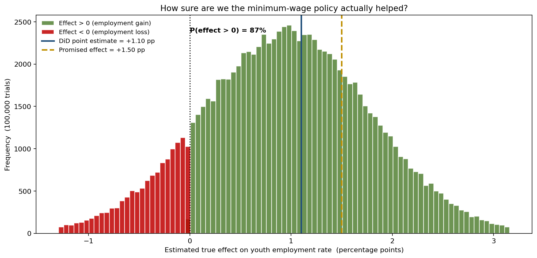
The naive reading — "the effect is +1.1 pp, it worked" — silently asserts the harm probability is 0% and the promise was nearly kept. The simulation says there is roughly a one-in-eight chance the policy backfired and a three-in-four chance it fell short of what was promised. Those are the numbers a minister defending the reform actually needs.

What effect size can the evaluation honestly certify?

A point estimate implies a step function: any claim at or below +1.10 pp is "supported," anything above is not. Uncertainty smears that step into a curve. Sweeping the claimed effect size and reading off the probability the true effect is at least that large turns the evaluation into a credibility curve.

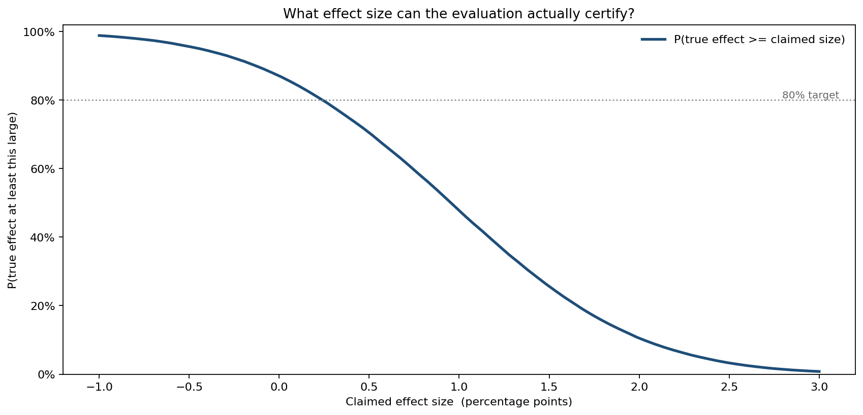
• A claim of +0.0 pp ("it helped at all") is supported with probability 87.1%.
• +0.5 pp: 70.4%.
• +1.0 pp: 47.8% — essentially a coin flip.
• The promised +1.5 pp: 25.6%.
• +2.0 pp: 10.5%.

The evaluation can credibly certify that the reform helped. It cannot credibly certify that it delivered the headline +1.1 pp, and it certainly cannot back the +1.5 pp promise. Reading the curve at the 80% confidence line shows the largest effect the study actually supports is well under half a point.

Where the doubt comes from — and why the SE understates it

Decomposing the spread of the true-effect estimate by source is where evaluation differs most sharply from a naive confidence interval.

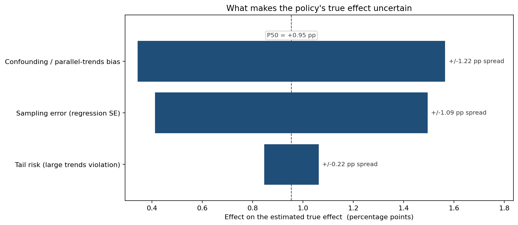
• Confounding / parallel-trends bias: ±0.61 pp (spread 1.22 pp)
• Sampling error (regression SE): ±0.54 pp (spread 1.09 pp)
• Tail risk (large trends violation): ±0.11 pp (spread 0.22 pp)

The single largest source of doubt is the one the regression standard error completely ignores. A conventional confidence interval is built from the 0.54 pp sampling component alone and would report a tidy ±1.06 pp band. Once the 0.61 pp confounding factor is admitted, the honest interval is materially wider — and asymmetric, because the bias is centred slightly negative. An evaluation that quotes only the regression SE is overstating its own certainty by ignoring its biggest unknown.

A point estimate hides the risk in every conclusion

Laying the naive reading beside the simulation makes the gap unmissable. The point estimate of +1.10 pp answers four yes/no questions with hard 100%/0% verdicts; the distribution attaches a real probability to each.

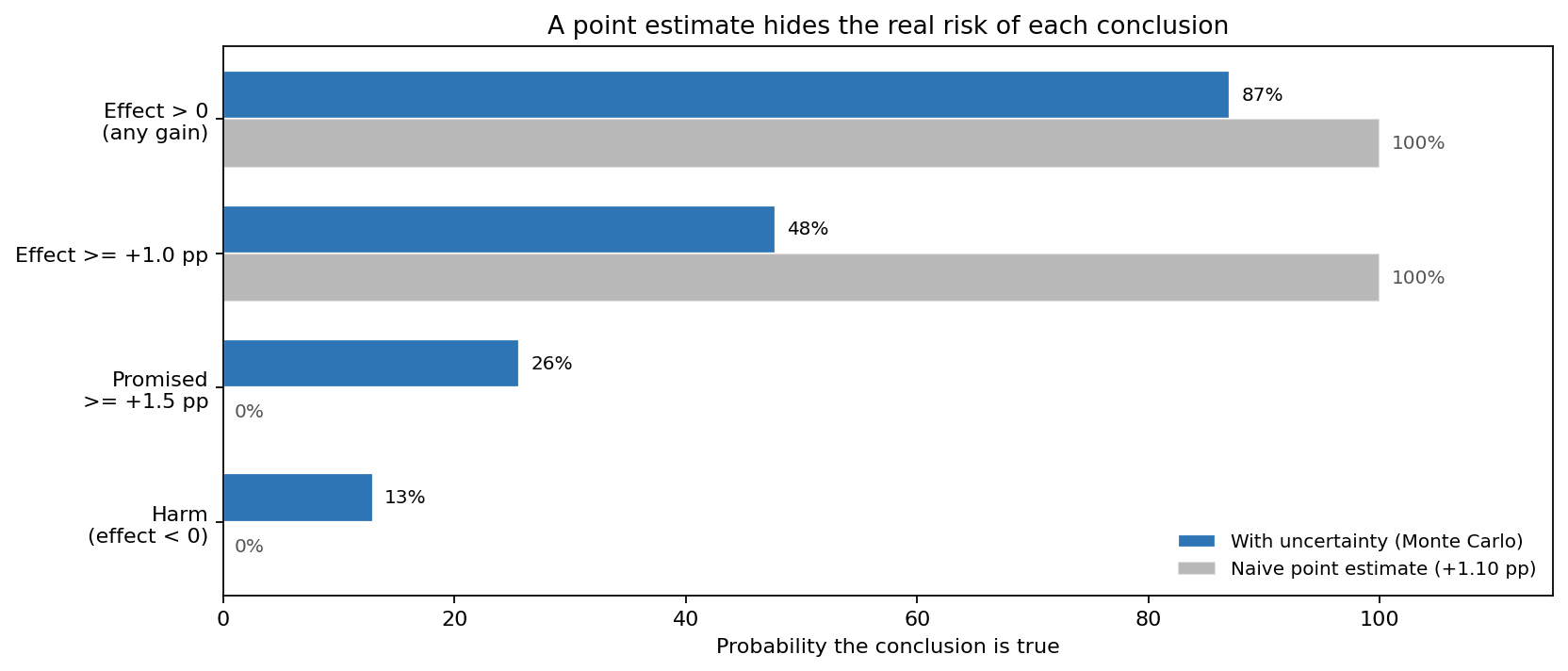
• Effect > 0 (any gain): naive 100% → true 87%
• Effect ≥ +1.0 pp: naive 100% → true 48%
• Promised ≥ +1.5 pp: naive 0% → true 26%
• Harm (effect < 0): naive 0% → true 13%

The point estimate is confidently wrong in both directions at once: it overstates the case for the policy having worked as advertised, while denying any possibility it harmed employment.

What the model changed

The evaluation unit had been about to report a clean success: "+1.1 pp, statistically significant." The simulation kept the verdict that the reform probably helped — 87% — but stripped out three false certainties. It put a 13% probability on the policy having actually reduced youth employment, a risk the headline buried. It showed the promised +1.5 pp had only a 26% chance of being real, tempering claims before they were made publicly. And it identified parallel-trends confounding, not sampling error, as the dominant source of doubt — pointing the next round of work toward a stronger control group rather than a larger sample.

ModelRisk functionality used

• Monte Carlo propagation of estimate uncertainty over 100,000 trials, converting the single +1.10 pp DiD coefficient into a full distribution of the true effect (mean +0.95 pp, 95% CI [−0.72, +2.60]).
• Layered uncertainty model combining a Normal sampling term (SE 0.55 pp) with a separate confounding/parallel-trends common factor and a heavy-tailed trends-violation shock — capturing the bias a regression SE cannot.
• Probability-of-conclusion outputs: P(effect > 0) = 87.1%, P(harm) = 12.9%, P(met +1.5 pp promise) = 25.6%.
• Credibility (power) curve sweeping the claimed effect size to show the largest effect the study can defend at 80% confidence.
• Tornado sensitivity ranking the uncertainty sources and exposing confounding (±0.61 pp) as larger than sampling error (±0.54 pp).
• Naive-versus-probabilistic comparison quantifying how a point estimate forces 100%/0% verdicts onto conclusions that genuinely carry 26–87% probability.

For an enacted policy, Monte Carlo turns evaluation from "the effect was +1.1 points" into "we are 87% sure it helped, 26% sure it met the promise, and 13% sure it backfired" — the distinction between reporting a coefficient and being honest about what it proves.