

Industry: Engineering
Product: ModelRisk
Application: Predicting Delivered Flow at a Pump-System Operating Point Under Hydraulic Uncertainty
The Hydraulic Calc Said 46 L/s Against a 44 L/s Demand. The Simulation Said One Build in Six Falls Short
A cooling-water loop was sized the way piping loops usually are: pick the pump, draw the system curve, find where they cross, read off the flow. The deterministic operating point came out at 46.4 L/s against a process demand of 44 L/s — a 5% margin, signed off as adequate. Then the commissioning engineer asked the question the single-point calculation cannot answer: given pipe-roughness scatter, fitting tolerances and pump-curve spread, how often does an as-built loop actually fall below 44 L/s? The Monte Carlo answer was 16% — roughly one build in six. A margin that looked comfortable on paper was a one-in-six commissioning failure.
The team rebuilt the operating point as a stochastic intersection in ModelRisk, solving the pump-versus-system balance for every simulated build and reading the delivered-flow distribution off the result.
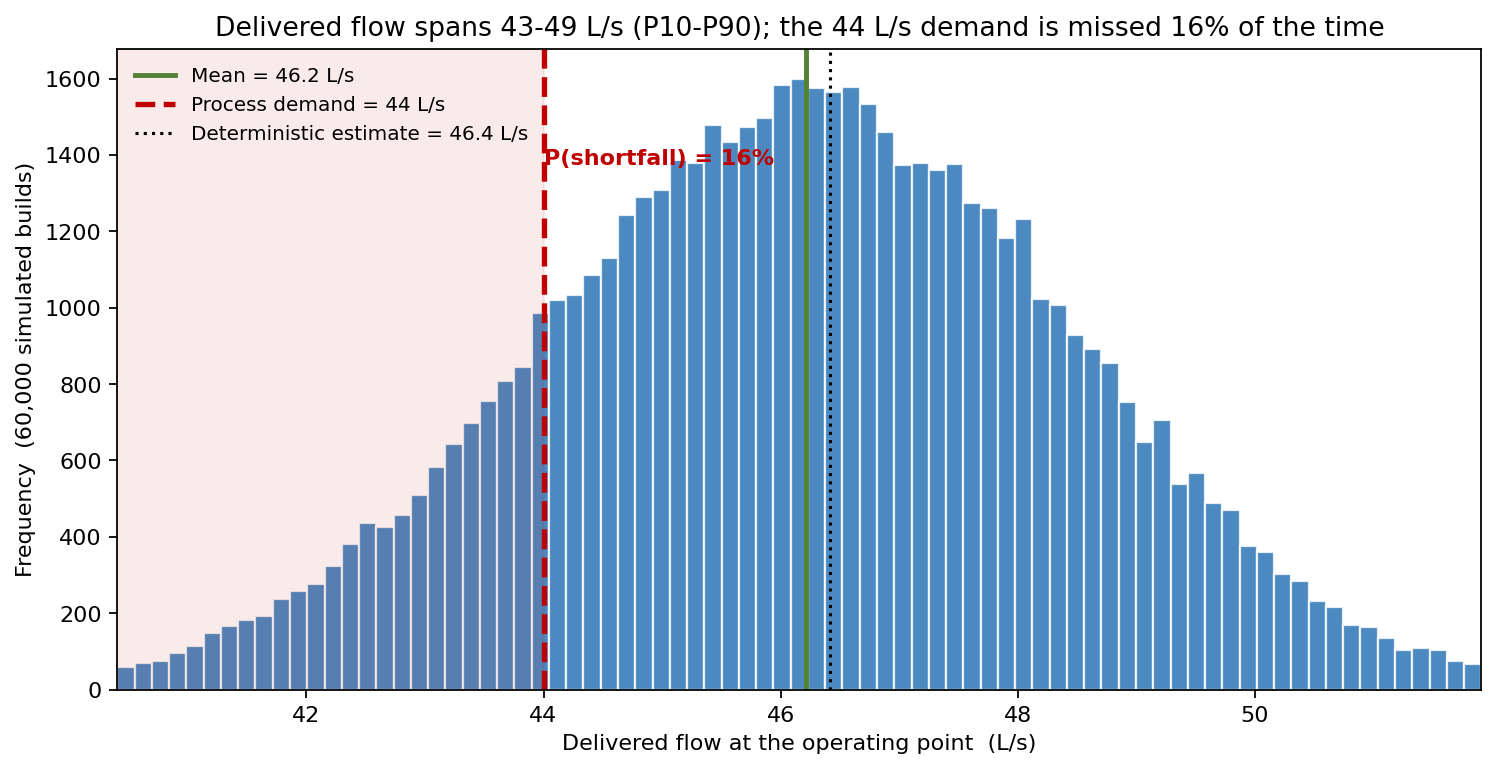
Across 60,000 simulated builds the delivered flow spans a P10–P90 of 43.3 to 49.1 L/s around a 46.2 L/s mean — and the left tail crosses the 44 L/s demand line often enough to give a 16% shortfall probability. The deterministic estimate (46.4 L/s, dotted) sits almost exactly on the mean, which is precisely why it is misleading: it reports the centre of the distribution and says nothing about the third of that distribution sitting closest to, and below, the requirement.
The operating point is an intersection of two uncertain curves
Delivered flow is not an input — it is the flow at which the pump's head equals the head the piping demands. The system head is the Darcy-Weisbach pressure loss plus static lift:
\[ H_{sys}(Q) = H_{static} + \left(f\frac{L}{D} + \sum K\right)\frac{V^2}{2g}, \qquad V = \frac{Q}{A} \]
and the pump head follows its catalogue curve \(H_{pump}(Q) = H_0 - aQ^2\). The operating point is the flow where \(H_{pump}(Q) = H_{sys}(Q)\), solved per trial by bisection. Each contributing input is uncertain:
- Pipe roughness ε — LogNormal around 0.08 mm median, feeding the friction factor f through the Haaland approximation to Colebrook. Roughness is non-negative and right-skewed (corrosion and poor finish only make it worse), so LogNormal, not Normal.
- Fitting K-values ∑K — LogNormal around 8.5 for the elbows, valves and entrance losses.
- Pump curve — shutoff head H₀ Normal at 32 ± 1.1 m and steepness a Normal, capturing build tolerance and impeller wear.
- Pipe inside diameter D — Normal at 150 ± 1.5 mm; because friction scales as roughly D⁻⁵ and velocity as D⁻², a small ID tolerance has outsized leverage.
A shared per-build install-quality factor scales roughness and fitting losses together: a sloppy install makes both worse at once. This keeps the inputs correlated rather than independent, which matters — treating them as i.i.d. would let their scatter cancel out and understate the tail.
Why a point estimate fails here
A single operating-point calculation propagates one value of each input and returns one flow. But friction is non-linear in roughness, the pump and system curves are both bands rather than lines, and the install-quality factor correlates the losses. The result is a delivered-flow distribution whose left tail — the only part that matters for "do we meet demand?" — is exactly what the nominal calculation throws away.
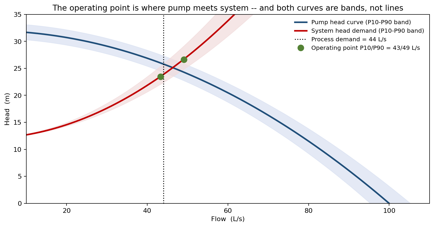
Both curves are uncertainty bands. At the 44 L/s demand flow the pump can produce a head of 24.2 to 27.2 m (P10–P90) while the system demands 22.5 to 26.0 m — the bands overlap, and where they cross is itself a distribution. The operating-point flow lands between 43.3 and 49.1 L/s (P10/P90). The deterministic calc picks the single crossing of the two median curves and reports it as fact.
Uprating the pump trades shortfall risk for erosion risk
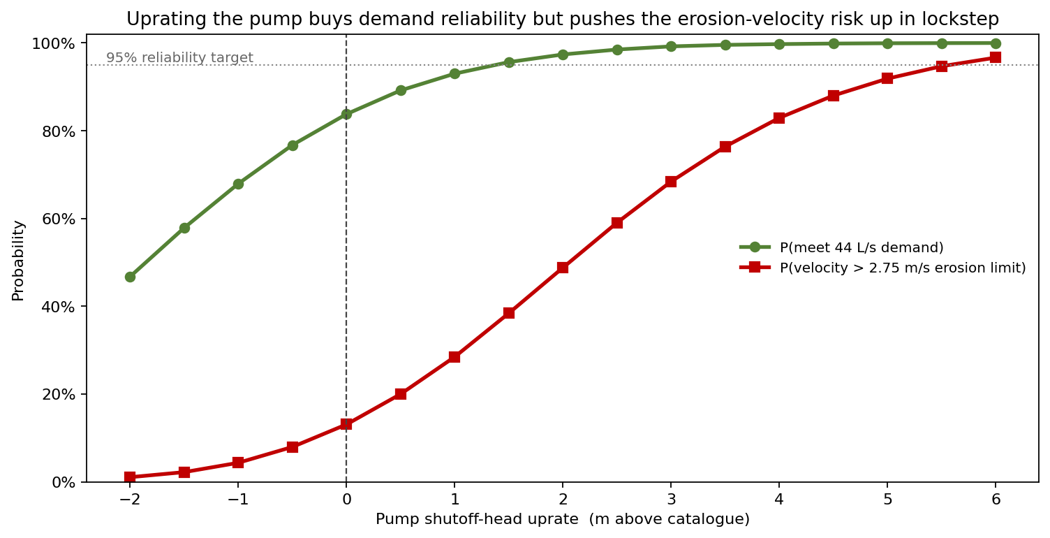
The obvious fix is a bigger pump — but more head means more velocity, and the loop has a 2.75 m/s erosion-corrosion velocity ceiling. Sweeping a shutoff-head uprate (a cheap impeller change) shows the two risks moving in lockstep:
| Shutoff-head uprate | P(meet 44 L/s) | P(velocity > 2.75 m/s) |
|---|---|---|
| catalogue (0 m) | 84% | 13% |
| +0.5 m | 89% | 20% |
| +1.0 m | 93% | 29% |
| +1.5 m | 96% | 38% |
| +2.0 m | 97% | 49% |
Reaching the 95% reliability target needs about +1.5 m of head — but that drives the erosion-velocity exceedance from 13% to 38%. The simulation makes the conflict explicit: you cannot buy demand reliability with head alone without paying in erosion risk. The eventual fix paired a modest +1.0 m uprate with a one-size-up section on the highest-velocity run, moving P(meet) to 93% while holding the velocity exceedance near 20%.
What actually moves the delivered flow
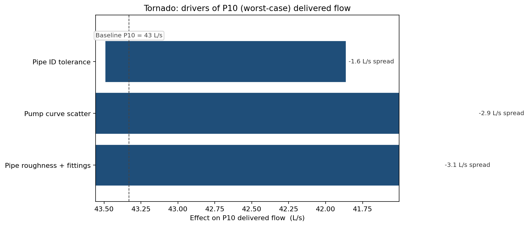
Ranking the drivers of the P10 (worst-case) flow, baseline 43.3 L/s:
- Pipe roughness and fittings are the largest lever — a rough, badly-fitted build costs about 2.1 L/s at P10 (3.1 L/s spread). This is where install quality control pays.
- Pump-curve scatter is a close second at 2.4 L/s on the downside — argument for a witnessed pump performance test rather than trusting the catalogue curve.
- Pipe ID tolerance is third at 1.6 L/s spread, small but not ignorable given its D⁻⁵ leverage on friction.
What the model changed
- Pump uprated +1.0 m and the highest-velocity run upsized, sized against the joint demand/erosion sweep rather than the single operating point — P(meet) raised from 84% to 93% without tipping the erosion-velocity risk past 20%.
- A witnessed pump performance test added to the procurement spec, after the tornado put pump-curve scatter neck-and-neck with roughness as a driver of worst-case flow.
- Install-quality acceptance (roughness and fitting count) tightened on the as-built loop, targeting the largest single P10 driver.
- The commissioning acceptance criterion rewritten as "P(flow ≥ demand) ≥ 95% across build tolerance" instead of "nominal flow ≥ demand", so the next loop is signed off against the distribution, not the midpoint.
ModelRisk Functionality Used
- Per-trial operating-point solver balancing the pump curve against the Darcy-Weisbach system curve by bisection, producing the delivered-flow distribution (P10–P90 of 43.3–49.1 L/s) instead of a single crossing.
- LogNormal roughness and fitting-loss inputs feeding the Haaland friction factor, correctly skewed and non-negative, rather than a Normal that would allow nonphysical negative roughness.
- Shared install-quality factor correlating roughness and K-values per build, preventing the independent-inputs cancellation that would have hidden the 16% shortfall tail.
- Uprate decision sweep quantifying the demand-reliability versus erosion-velocity trade — showing +1.5 m of head buys 96% reliability but a 38% erosion exceedance.
- Tornado on P10 flow identifying pipe roughness/fittings (−2.1 L/s) and pump-curve scatter (−2.4 L/s) as the controlling worst-case drivers, directing the spec changes.
A nominal operating point tells you where the loop runs on an average day with an average build. The delivered-flow distribution tells you how often the loop you actually built will miss its demand — and Monte Carlo is what gets you from the first answer to the second.