Industry: Energy
Product: ModelRisk
Application: Energy procurement under uncertainty

Hedging a 4.8 TWh Annual Load: Energy Procurement with ModelRisk

A North American specialty-chemicals group consumes 4.8 TWh of electricity and 14 million MMBtu of natural gas per year across eleven plants. At a baseline spot price of $58/MWh and $3.40/MMBtu, the annual energy bill runs about $326M — roughly 18% of cost of goods sold. A $10/MWh move on power alone shifts EBITDA by $48M. The procurement team's job is not to forecast prices; it is to shape the distribution of next year's energy bill so that the 95th-percentile outcome stays inside the budget envelope set by the CFO. That is a Monte Carlo problem, not a spreadsheet problem — and once each candidate hedge book is run as a full cost distribution, the strategies that look identical on an expected-cost line separate sharply in the tail:

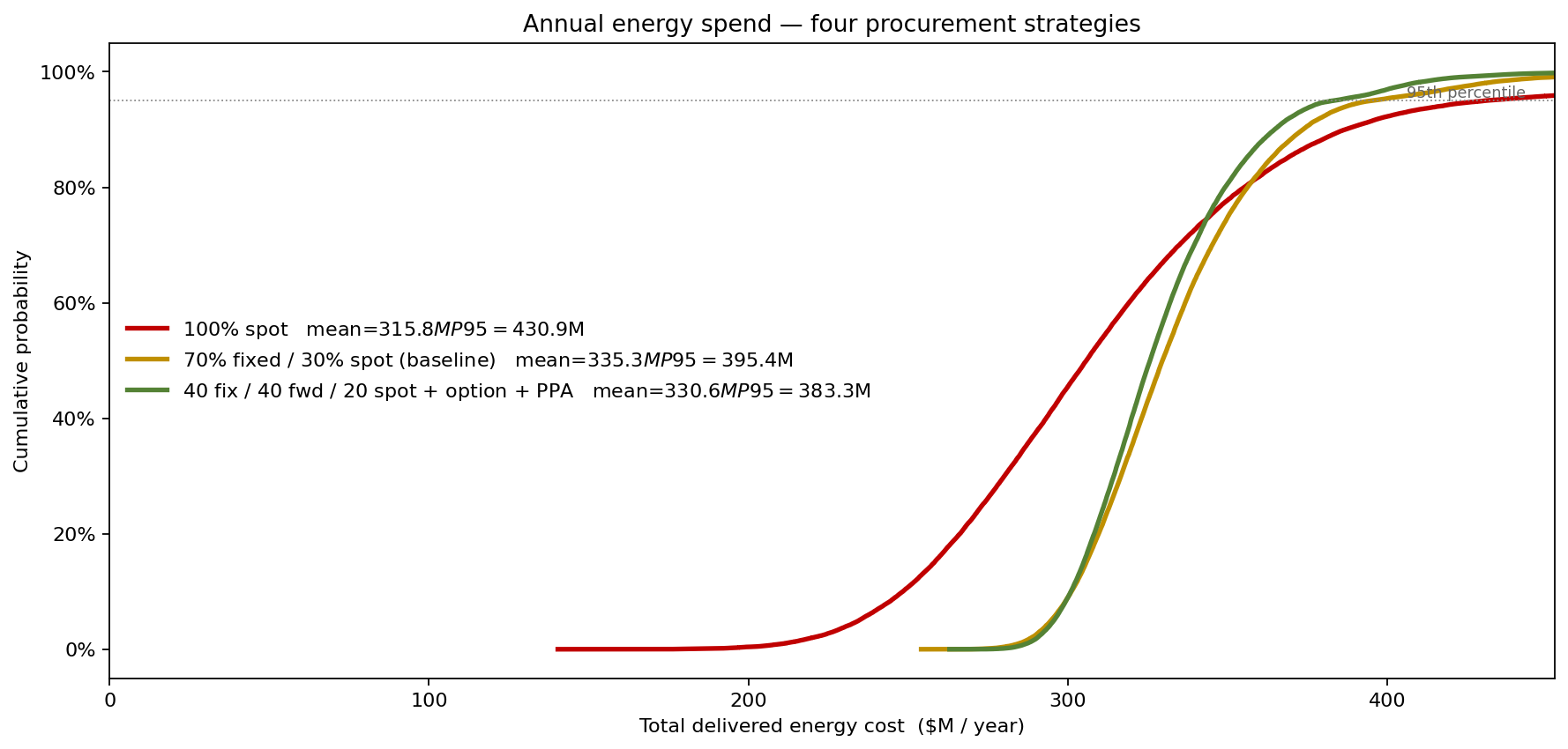
Pure spot exposure has the lowest mean (about $316M) but a 95th-percentile bill of $431M; the layered Strategy 4 pays roughly $15M more in expected cost to pull that 95th percentile down to $383M. The rest of this study is about where that tail comes from and how much it costs to compress.

Where the price uncertainty actually lives

Wholesale power prices in PJM and ERCOT exhibit three structurally different behaviours that must be modelled separately rather than smeared into a single Geometric Brownian Motion. GBM assumes constant volatility and no jumps — which is wrong on every count for power.

Body of the on-peak distribution. Hourly on-peak LMPs over the past three calendar years fit well to a LogNormal with median $52/MWh and σ on the log scale of 0.34 — a coefficient of variation of about 36%, matching observed annualised volatility for ERCOT-North.

Scarcity spikes. ERCOT clears at the $5,000/MWh price cap on roughly 35 hours per year (0.4% of the time). These are not GBM tails; they are a separate compound-Poisson regime triggered by reserve scarcity. The model uses a Poisson rate λ = 35 hours/year with severity drawn from a Generalized Pareto above the $250/MWh threshold (ξ = 0.42, scale 180). Lumping these into a single lognormal under-prices the tail by an order of magnitude.

Natural-gas linkage. Henry Hub gas was modelled as a mean-reverting Ornstein–Uhlenbeck process in log-price with long-run mean $3.40/MMBtu, half-life 8 months, and annual vol 38%. Power and gas were tied with a Gaussian copula ρ = 0.62 in the body and a t-copula with ν = 4 in the upper tail — gas-fired marginal units mean the two markets co-spike during scarcity events, and a Gaussian copula alone misses that.

Four procurement strategies, one cost distribution each

The team modelled the next 12 months under four mixes:

1. 100% spot — pure exposure.
2. 70% fixed at $61/MWh, 30% spot — the historical baseline.
3. 40% fixed + 40% 12-month forward strip at $60.20 + 20% spot.
4. Strategy 3 plus a $80/MWh call option (10% of load, premium $2.40/MWh) and a 15-year solar PPA for 8% of load at $42/MWh fixed.

Each strategy was scored on total delivered cost over 50,000 simulated years (the four-way cost comparison is the chart above).

The deterministic forecast said all four strategies cost within $3M of each other — there was no apparent reason to prefer one. The simulation said otherwise: 100% spot has a mean of $316M but a 95th percentile of $431M, while the layered Strategy 4 has a mean of $331M (about $15M higher) and a 95th percentile of $383M — $48M of tail compression for a $15M premium. The decision criterion is no longer "lowest expected cost"; it is "lowest 95th percentile subject to mean ≤ $335M", and that frame is only legible once you have the distribution.

What actually moves the bill

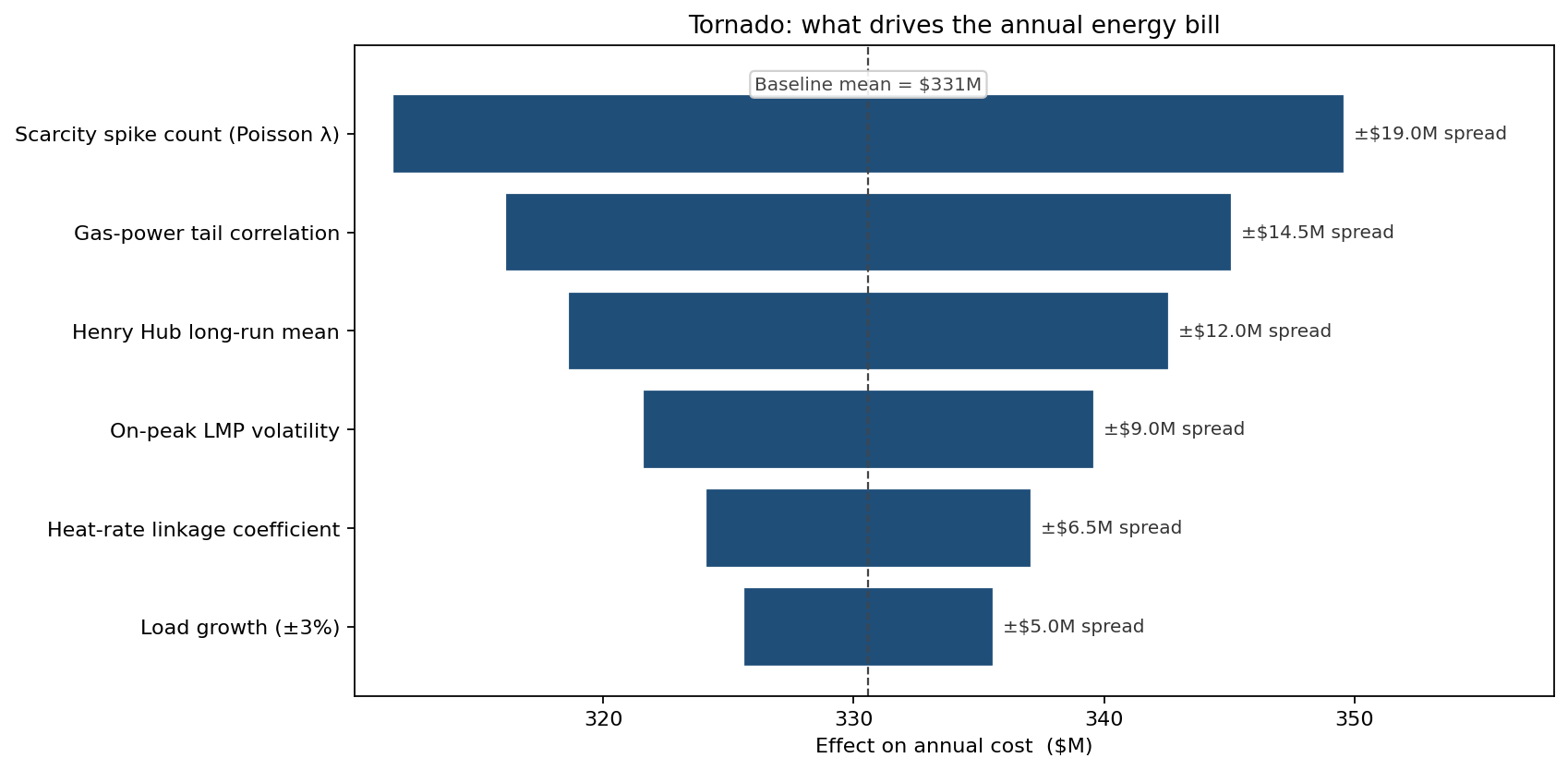
Scarcity-spike count dominates — a single year with 60 cap hours instead of 35 adds $19M independent of average price. Gas–power tail correlation is second; this is the term most often dropped from in-house spreadsheets, and dropping it understates the 99th-percentile cost by roughly $24M.

Hedge ratio sweep

The hedge ratio (% of load locked in fixed) was swept from 0% to 100% in 10-point steps, plotting mean and 95th-percentile cost for each.

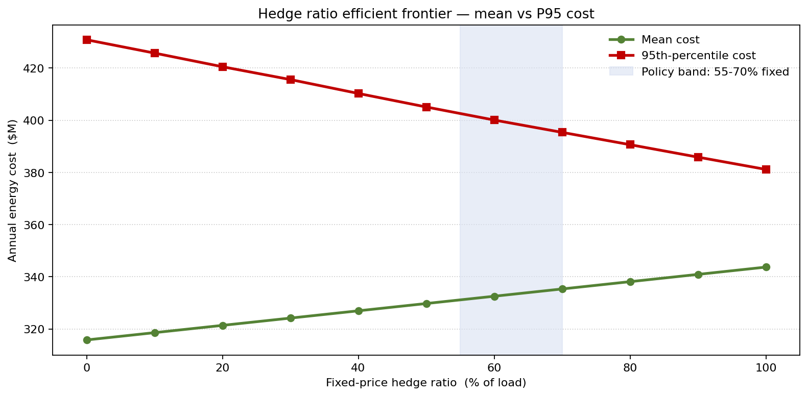
The classic efficient-frontier shape emerges: moving from 0% to 60% fixed cuts the P95 by $31M for an expected-cost penalty of $17M. Beyond 70%, additional fixing buys steadily less tail reduction per dollar of expected-cost penalty and starts adding a "regret" left tail in scenarios where spot collapses. The team set a policy band of 55–70% fixed, reassessed quarterly.

What changed

• Hedge book restructured: moved from 70% fixed / 30% spot to a layered 40% fixed / 40% forward strip / 20% spot + option overlay + PPA. Expected cost up $15M; P95 cost down $48M.
• Budget variance band tightened: 90% confidence interval on next year's spend narrowed from ±$98M to ±$44M, materially easing the dialogue with treasury and the audit committee.
• PPA case made on tail value, not LCOE. The solar PPA was rejected three years running on a simple LCOE comparison; the simulation showed it pays for itself purely as a hedge against gas–power co-spikes during summer peak.
• Procurement KPI redefined from "actual vs forecast price" (an unwinnable game) to "actual cost inside the modelled 90% CI" — a target the team can hit and the board can audit.

ModelRisk Functionality Used

• Compound-Poisson with Generalized Pareto severity for ERCOT scarcity spikes — modelled separately from the lognormal body of the on-peak price distribution.
• Ornstein–Uhlenbeck mean reversion for Henry Hub gas with calibrated 8-month half-life.
• t-copula in the upper tail linking power and gas (ρ = 0.62, ν = 4) — Gaussian-only coupling missed ~$24M of 99th-percentile cost.
• Strategy comparison via overlaid CDFs, scoring mean and P95 jointly rather than mean alone.
• Hedge-ratio sweep producing the mean-vs-P95 efficient frontier that set the 55–70% fixed-load policy band.
• Sensitivity ranking that identified scarcity-hour count and gas–power tail correlation as the two terms most worth investing modelling effort in.

For a buyer this size, hedging is not a bet on the price forecast — it is the explicit purchase of distribution shape. Monte Carlo simulation in ModelRisk is what makes that shape tradeable.