Industry: Energy
Product: ModelRisk
Application: Measurement & Verification of Energy Efficiency Savings

When the Retrofit Saved 24% and the M&V Said 9%: Quantifying Baseline Uncertainty in Energy Efficiency Projects

A $14M chiller-plant retrofit at a 1.2M sqft commercial campus was designed to cut cooling-energy use by 28% against the prior-three-year baseline. After 12 months of post-retrofit operation, the IPMVP Option C measured saving — adjusted for weather and occupancy — came in at 24%. The performance contract paid out on a measured saving of 9.4%, because the baseline-regression confidence interval covered the difference. The owner was furious, the ESCO was furious, and the engineering team was right: the uncertainty in the baseline was bigger than the uncertainty in the retrofit.

A facilities-engineering team rebuilt the M&V framework in ModelRisk for the next round of retrofits — six buildings, $48M committed capex — to make the uncertainty band on measured savings explicit before the contract was signed, not after the first reconciliation invoice. The headline output was a full distribution of measured savings — the picture the single deterministic 28% point estimate could never show.

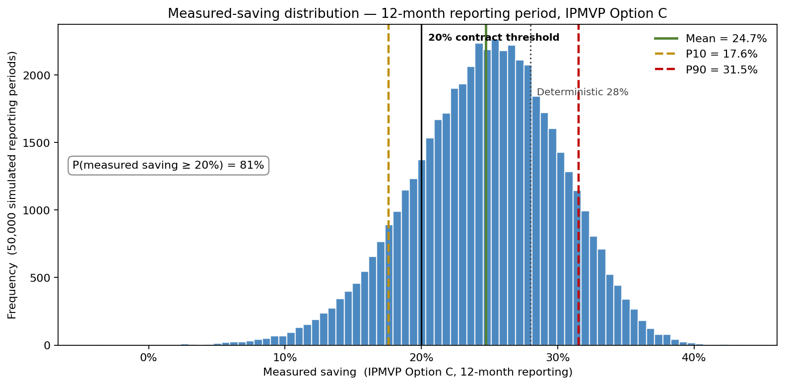
The simulated measured saving has a mean of 24.7% with P10 = 17.6% and P90 = 31.5%, and clears the contractual 20% threshold in 81% of futures — not the certainty the deterministic 28% implies. The width of that band, not its centre, is what drives the contract design that follows.

The IPMVP baseline is a regression, not a number

The standard M&V protocol (IPMVP Option C) fits a regression of monthly energy use against weather (cooling degree days, heating degree days) and operational drivers (occupancy hours, production volume). Savings are the difference between predicted baseline and measured post-retrofit consumption, and uncertainty in that difference is dominated by:

• Regression residual standard error (σ_reg) — typical 4–7% of predicted baseline for a well-calibrated commercial building, larger when the baseline period was atypical weather.
• Weather variability in the reporting year — coefficient on CDD has uncertainty σ_CDD ≈ 8%; a hot summer pushes the predicted baseline up and the measured saving down.
• Occupancy drift — a building with 5% more occupancy in the reporting year shows lower apparent savings; this is captured imperfectly by a single linear term.

For the campus, the deterministic point estimate said expected savings = 28%, with a "± 3% engineering judgement" footnote. The Monte Carlo reframing instead simulates the joint distribution of (baseline-regression coefficients, reporting-year weather, occupancy drift, equipment performance variance) and produces a full distribution of measured savings:

\[ \text{Saving}_{\text{measured}} = 1 - \frac{E_{\text{post}} + \epsilon_{\text{meter}}}{\hat{\beta}_0 + \hat{\beta}_1 \text{CDD} + \hat{\beta}_2 \text{HDD} + \hat{\beta}_3 \text{Occ}} \]

with the β coefficients drawn from their joint posterior (multivariate Normal with the regression covariance matrix) and weather/occupancy drawn from their own distributions.

As the distribution above shows, the result is mean measured saving 24.7%, P10 = 17.6%, P90 = 31.5%. The deterministic 28% sits at the 72nd percentile. The contractual threshold for full performance payment (≥ 20%) is met in 81% of futures, not the 100% the deterministic estimate implies.

Performance contract redesign

The original contract had a binary threshold: ≥ 20% measured saving → full payment, otherwise nothing. The risk distribution made the binary structure dangerous for both sides: a 19% probability of zero payment in good-faith retrofits, and a real probability the ESCO walks away with full payment on a retrofit that only delivered 16% of true savings (high-baseline year).

A redesigned contract pays linearly on a banded structure:

• 0–15% measured: zero payment.
• 15–20%: ramped 0–100% of fee.
• 20%+: 100% of fee + 50% gain-share on excess up to 32%.
• A 24-month moving-average reporting period rather than 12, which cuts σ_reg by roughly √2.

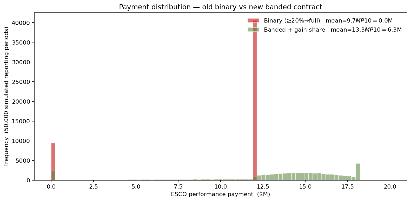
Under the new structure: expected payment to ESCO is $13.3M against the old expected $9.7M, but the P10 payment is $6.3M against the old $0. The variance to both sides collapsed, the dispute risk fell out of the contract, and the gain-share term gave the ESCO incentive to over-perform on the next batch of measures.

What drives the measured-saving uncertainty

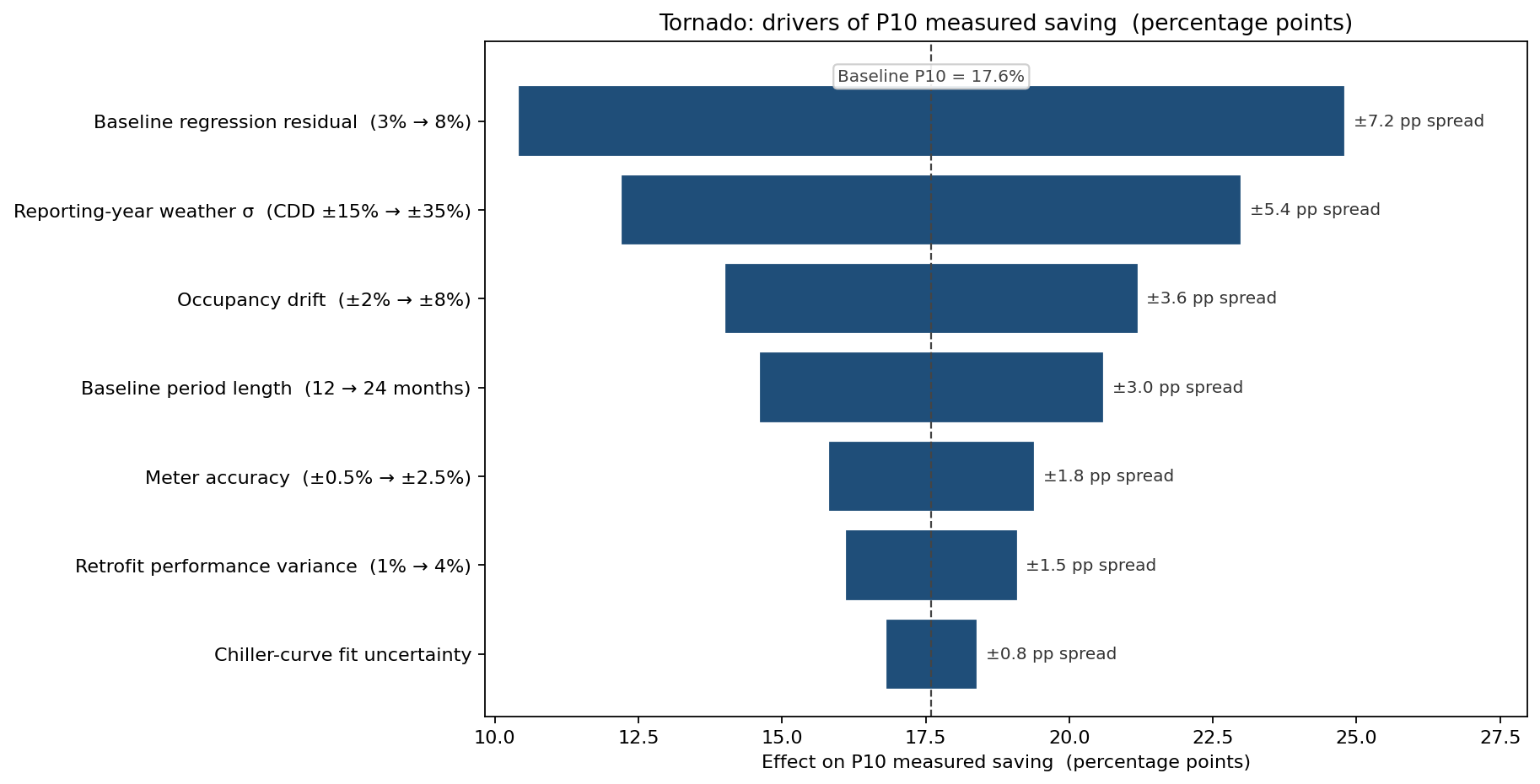
The largest single driver is baseline regression residual — the noisy fit between historical kWh and degree-days. A second-year-of-baseline addition collapses σ_reg by 30–40% and shifts the P10 saving up by 4.7 percentage points, more than any retrofit-design change available. Reporting-year weather variability is second; the model recommended a 3-year moving-average normalisation rather than a single year, with the trade-off that the project ROI signal is delayed.

The metric that the deterministic team had spent most engineering hours refining — the chiller-plant efficiency curve — ranked sixth: the equipment is well-characterised, the baseline is not.

What changed

• 24-month reporting period with a 3-year moving-average weather normalisation, baked into the M&V plan instead of the 12-month default.
• Performance contract restructured to a banded payment with explicit gain-share above 20% measured saving, cutting both parties' variance.
• Baseline data investment: a second year of pre-retrofit submetering added to the next four projects in the portfolio, at $180k cost, which the simulation valued at $1.4M in expected payment-dispute avoidance.
• Stopped paying for redundant chiller-curve characterisation — the ranking showed it moved P10 saving by less than 0.8 percentage points, against budgets in the high six figures.

ModelRisk Functionality Used

• Multivariate-Normal draws of baseline regression coefficients from their estimated covariance matrix, which is the statistically correct way to propagate fit uncertainty into the savings figure — not the "± engineering judgement" the deterministic plan used.
• Joint simulation of weather and occupancy with calibrated correlation (a hotter year is also a higher-occupancy year in this building stock), so that the reporting-year scenario is internally consistent.
• Custom payment-function logic in Excel for the banded contract, evaluated against each simulated saving outcome.
• Tornado on P10 measured saving rather than mean, because contract design is determined by the lower tail and the driver ranking on P10 is different.
• Comparison of 12 vs 24-month reporting as a direct overlay of two saving distributions on the same set of underlying simulated outcomes.

In efficiency M&V, the uncertainty in the savings figure is dominated by the baseline, not by the technology. Monte Carlo simulation puts a number on that uncertainty before the contract is signed — which is the only place the number can usefully be used.