Industry: Construction and Infrastructure
Product: ModelRisk
Application: Workforce Allocation — Crew Sizing Under Productivity Uncertainty

Hiring two extra crews looked wasteful. The probability of needing them was 38%.

A $410M highway widening project planned a peak workforce of 240 craft workers across 14 trade specialities. The deterministic earned-value plan said the crews were sized at 105% of expected demand — a 5% cushion against productivity variability. The Monte Carlo on the same productivity inputs said there was a 38% chance of needing 18 more workers than planned in at least one peak month, and a 12% chance of needing 35 more. Hiring those workers reactively cost roughly 1.8× the price of having them on the books from the start. Sized for the mean, the workforce was structurally under-resourced for the upper half of the distribution.

A specialty contractor adopted ModelRisk to convert the labour-loaded schedule from a deterministic earned-value plan into a probabilistic crew-sizing model.

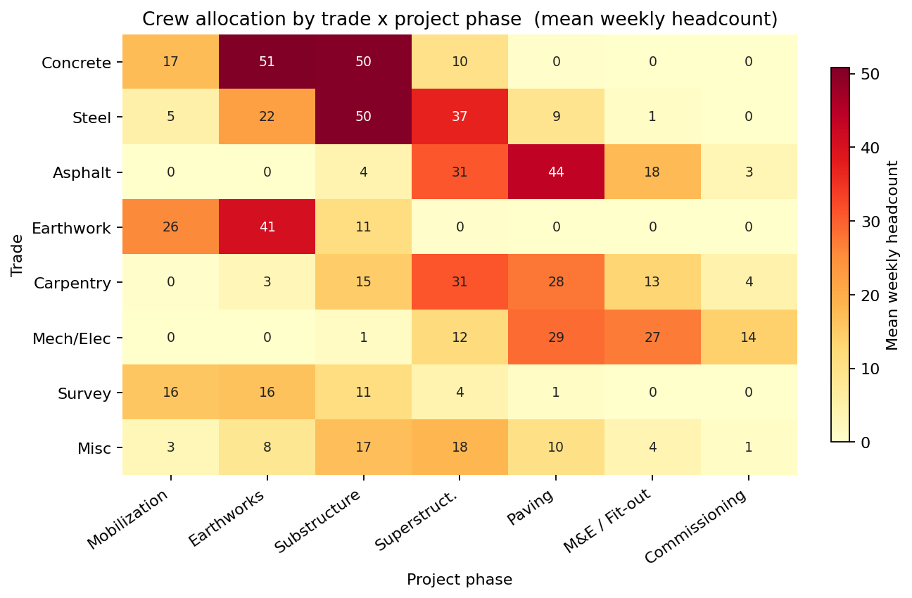
The labour-loaded schedule allocates each trade across the project phases. Aggregating the planned weekly headcount by trade and phase shows where the crews concentrate — and where the peak contention sits, as concrete, steel and earthwork all load into the substructure and superstructure phases at once:

Productivity is a distribution, not an input

The deterministic plan used a single productivity factor per trade — derived from the firm's earned-value benchmark of 0.93 units per crew-hour on similar projects. The Monte Carlo replaced this with calibrated distributions:

• Concrete placement — Beta(α=4, β=3) on the 0.85–1.09 range, mean ≈ 0.99. The Beta captures the bounded nature of productivity (cannot be negative or unboundedly high) and the slight left-skew from bad-day clustering.
• Steel reinforcement — Beta(α=3, β=4) on 0.82–1.08, lower mean and higher variability — the bar-bending trade had more dispersion in the historical record.
• Asphalt paving — Triangular(0.87, 1.00, 1.13) — temperature-sensitive, slightly right-skewed because exceptional days happen but bad days cap at the weather threshold.
• Earthwork / excavation — Lognormal-scaled, median 0.98, σ_log 0.09 — right-skewed by ground-condition surprises.

The absenteeism rate was modelled as Beta(α=2, β=46) (mean 4.2%, calibrated to the contractor's HR records over 23 prior projects). Weather lost days were modelled as Negative Binomial (mean 14/quarter, k=2) — clustered, not Poisson.

What "P95 crew demand" looks like across the schedule

The simulation stepped weekly through the 18-month project, drawing trade-specific productivities and absenteeism each week, computing the required crew complement to meet the schedule, and recording the peak across the project. The peak weekly workforce came out as:

• Deterministic peak 240 workers.
• Mean peak 246 workers.
• P75 peak 268 workers.
• P95 peak 294 workers.
• P99 peak 301 workers.

The deterministic plan of 240 sat just below the median of the simulated peak distribution — a roughly 54% probability that the planned crew complement would be insufficient at some point in the project. Reframing the sizing decision as a confidence curve makes the trade-off explicit: the sweep below plots P(crew meets every milestone without a reactive hire) against standing crew size. Reaching 90% milestone confidence required about 288 workers, while the planned 240 bought only ~46%.

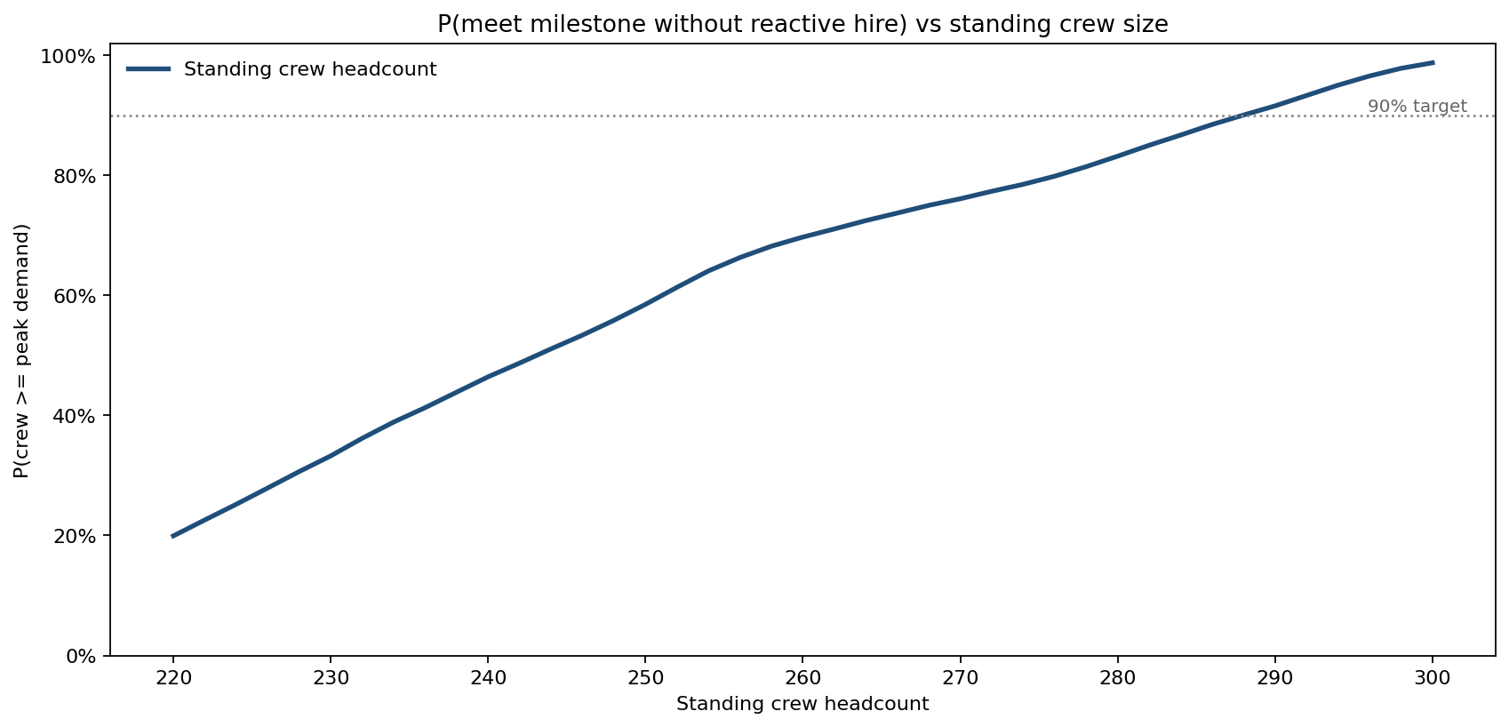
The labour-rate spread between planned-headcount cost ($28/hr loaded) and reactive-hire premium cost ($50/hr through agency) made the cost of being wrong about peak demand substantial.

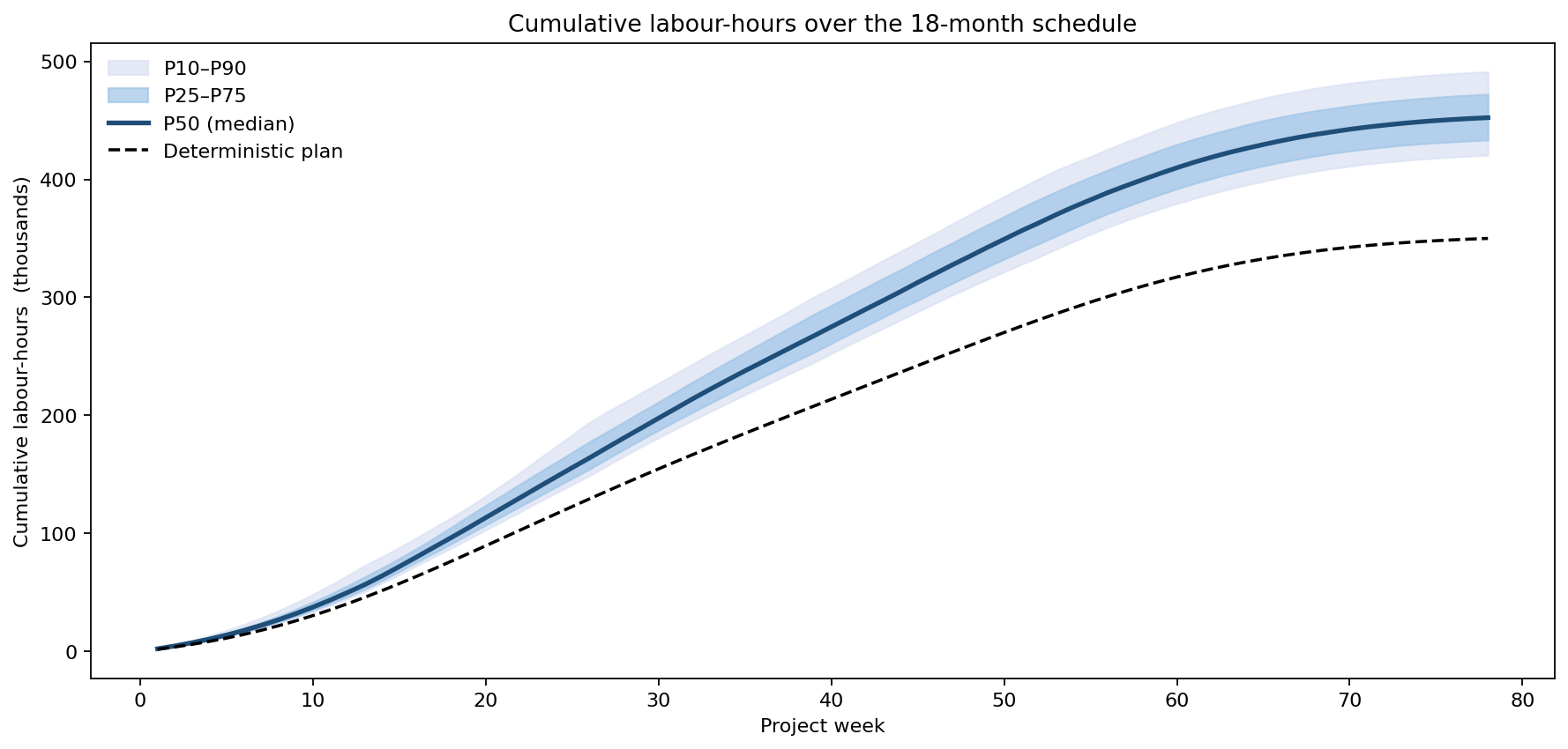
The same uncertainty accumulates over the whole schedule. The fan chart below tracks cumulative labour-hours week by week: the deterministic plan lands near 350k hours, while the simulated P50 reaches ~452k and the P90 ~491k — the gap is the labour the deterministic plan never budgeted for.

Three crew-sizing policies, three cost curves

Three policies were compared:

• Baseline — planned headcount 240, agency-hire fills any shortfall.

• +10% buffer — planned 264, agency for residual shortfall.

• Hybrid — planned 240 + standing 30-worker subcontract option (no commitment cost, exercised in 2-week blocks at a 12% premium over loaded rate when the demand forecast exceeds threshold).

• Baseline — mean labour cost $19.4M, P90 $22.1M.

• +10% buffer — mean $20.8M, P90 $21.9M. Tighter distribution, higher expected cost.

• Hybrid — mean $19.1M, P90 $20.4M. Lowest expected cost AND lowest P90 — option value paid for itself.

The Hybrid policy was selected. It cost slightly more than the headline Baseline in the median case, but the tail was 23% shorter, and the avoided agency-premium tail was $1.7M at the P90.

Which inputs drive the answer

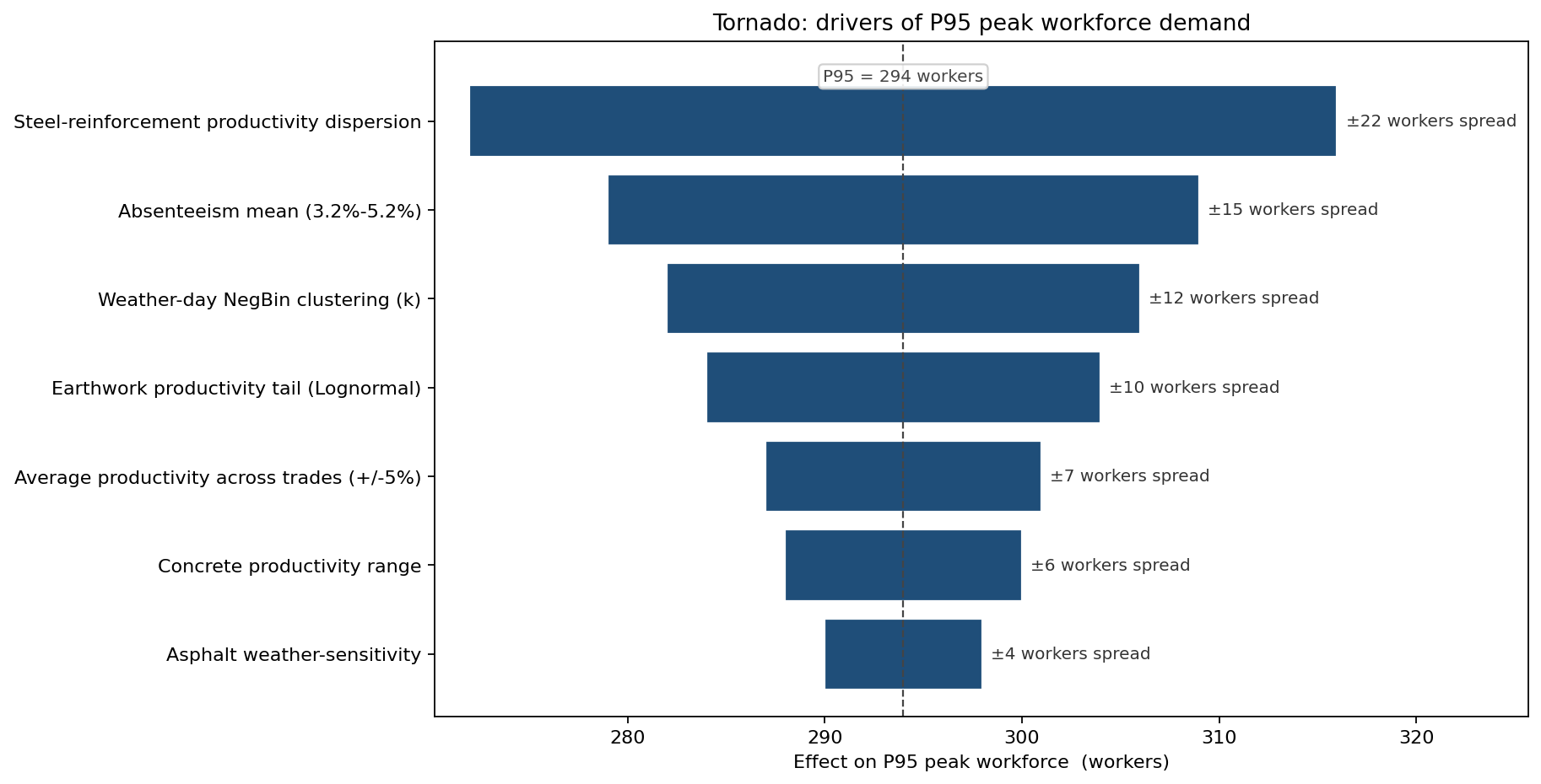
The biggest mover of P95 peak was the steel-reinforcement productivity dispersion — the trade with the widest historical productivity range was also the trade with the largest contribution to peak-week demand. Second was absenteeism mean (a 1pp swing on the 4.2% baseline moved P95 by 11 workers). Third was the weather-day clustering parameter — clustered weather pushed multiple trades into the same recovery window, which a Poisson misses entirely.

Surprisingly low on the tornado was the average productivity across trades — moving the mean by ±5% had a smaller effect on P95 than moving the dispersion did. The contractor had been chasing average-productivity improvements through training programmes; the model said the higher-leverage investment was in dispersion-reduction programmes (better tooling, prefab kitting, standard methods) that compress the lower tail of bad days.

What the model changed

The contractor signed the standing subcontract option, restructured the steel-rebar trade to use a prefab cage assembly that compressed the lower productivity tail by 15%, and built a weekly "look-ahead" trigger that exercised the subcontract option when the 4-week forecast peak demand exceeded 248 workers. The realised peak workforce reached 252 in week 38; the subcontract option was exercised for 6 weeks. Realised labour cost over the project came in at $19.0M, inside the P40 of the Hybrid policy's distribution and $1.1M below the Baseline policy's expected cost. The subcontract premium of $0.18M was recovered 9× by avoided agency premiums.

ModelRisk Functionality Used

• Trade-specific productivity distributions (Beta, Triangular, Lognormal) calibrated from 23 prior projects — replaced the single 0.93 earned-value factor.
• Weekly resampling over 18 months captured the peak-week distribution that monthly or quarterly aggregation collapses.
• Negative Binomial weather days modelled storm clustering correctly — Poisson under-stated cross-trade contention by 14%.
• Option-value comparison of the Hybrid subcontract trigger versus +10% planned headcount showed the option was both cheaper in expectation AND tighter in the tail — a Pareto improvement.
• Sensitivity ranking identified productivity dispersion (not mean) as the dominant driver of P95 peak demand, redirecting capability investment from training programmes to dispersion-reduction methods (prefab, kitting, standard cells).
• Trigger-rule integration turned the simulation from a sizing exercise into a live operational rule that recovered $1.6M of avoided agency premium across the project.

In workforce planning, the average is the headline number and the dispersion is the budget driver. Monte Carlo is what turns dispersion from a footnote into a decision input.