Industry: Construction and Infrastructure
Product: ModelRisk
Application: Project Cost Estimation

Where the $2.5B transit deterministic estimate actually lived

A $2.5B subway extension was approved on a deterministic Class 3 estimate. Run as a Monte Carlo against the same cost breakdown, the same numbers produced a P50 of $2.82B, a P90 of $3.35B, and an 85% probability of overrunning the headline budget. The deterministic estimate was not the most likely cost — it was the mode of one cost driver, multiplied by the mode of the next, multiplied by the mode of the next. The product is almost never the modal outcome.

ModelRisk was brought in to replace the spreadsheet "best case + 10%" contingency with a probabilistic cost stack the project board could defend to a transport ministry.

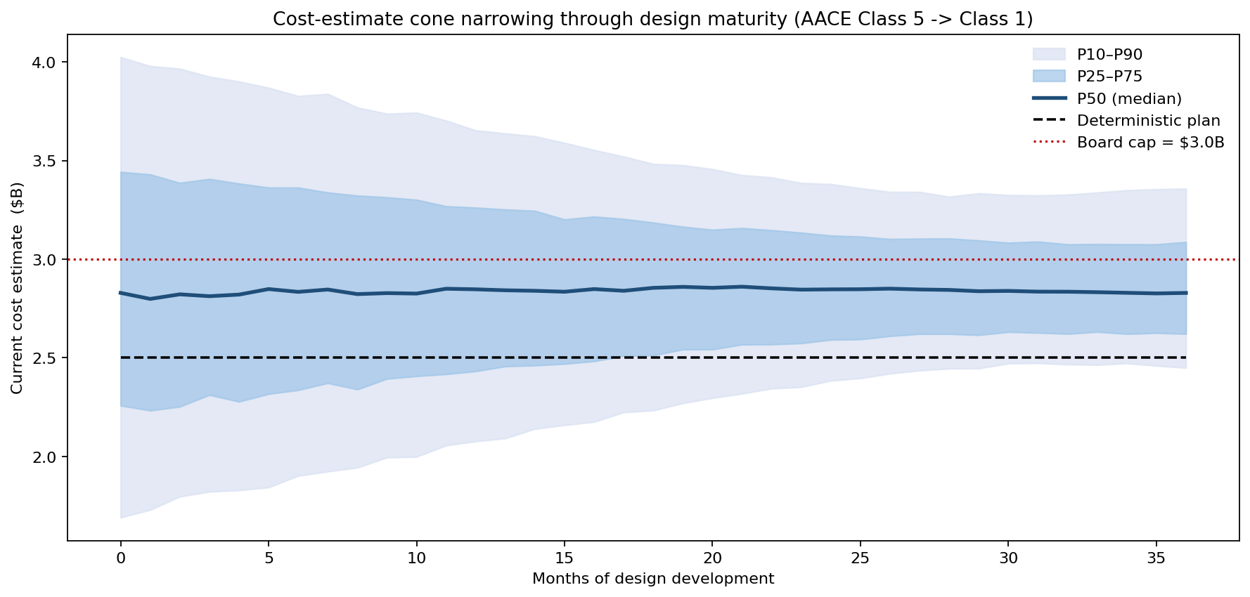
The AACE estimate cone shows how the estimate width should narrow as design develops. At month 0 (Class 5, conceptual) the estimate width is roughly ±50% — any number in $1.5B–$3.5B is defensible. Through Class 4 (FEL2), Class 3 (FEL3, basis for funding), Class 2 (control estimate) and Class 1 (post-bid) the cone tightens, but the centre drifts upward toward the simulated mean ($2.87B), not toward the deterministic $2.50B that anchored the Class 3 funding request. By month 36 the cone has closed around the realised value — but the $3.0B board cap (red dashed line) is breached by the upper edge of the cone from Class 4 onward. The Monte Carlo says the board cap was too tight even at the design class it was set against.

Distributions, not point estimates, for every line in the cost stack

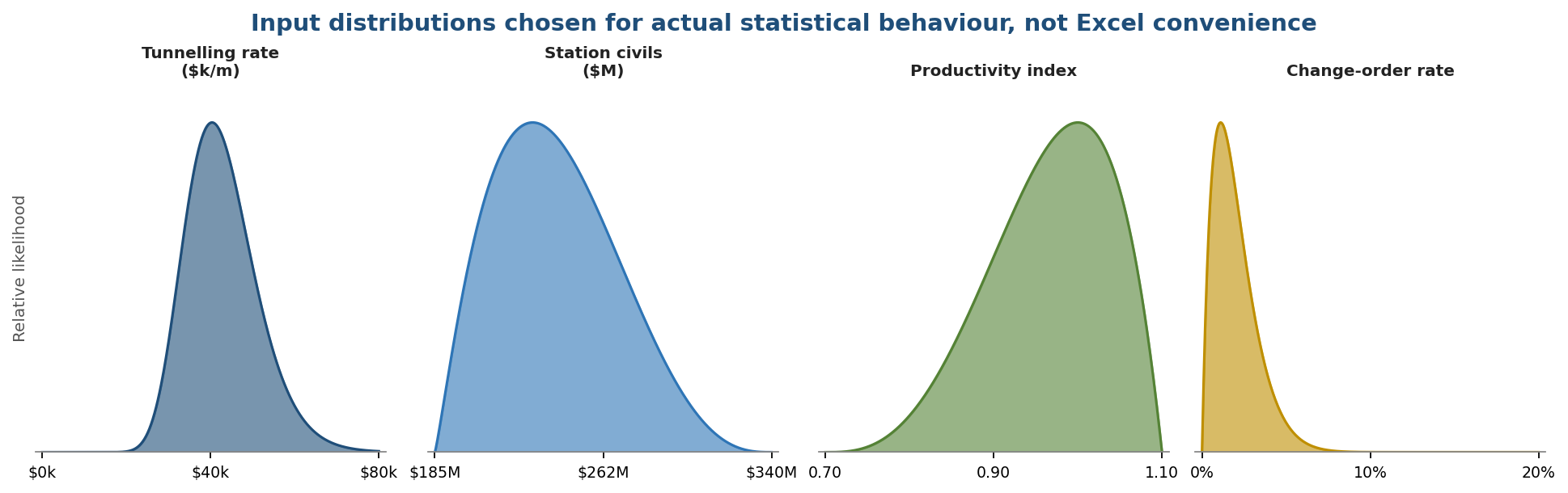
The Class 3 estimate had ~140 line items rolled up into six categories: tunnelling, stations, trackwork, systems, professional services, and contingency. Each line was re-cast as a distribution chosen for its actual statistical behaviour, not Excel convenience:

• Tunnelling unit rate — LogNormal, median $42k/m, P90 $58k/m. Bore rates skew right because the bad month (squeezing ground, cutter-head change-out) dominates the average.
• Station civils — PERT(min $185M, mode $230M, max $340M). The upside tail accounts for late architectural change orders, which historically have run 8–14% of station scope on this metro system.
• Steel and copper indices — geometric Brownian motion with annual drift 2.5% and volatility 18%, sampled monthly across the 5-year construction window. Long-dated procurement locks were modelled as a separate path; the unlocked exposure ran 32% of metal spend.
• Labour productivity — Beta(α=4, β=2) on output index between 0.70 and 1.10, calibrated to the firm's own benchmarking database across 17 prior metro projects.
• Weather-loss days — Negative Binomial (mean 22 days/year, k=3) rather than Poisson. Bad weather clusters; a Poisson fit understated the P95 by 40%.
• Change-order rate — Beta(α=2, β=18) scaled to the 0–20% range, with mean 10% — matching the industry 5–15% norm.

The total cost was assembled by summation, with a Gaussian copula imposing a 0.55 correlation between tunnelling and station civils (shared labour pool), and 0.40 between steel index and trackwork (rebar and rail are the same commodity in different shapes).

What 50,000 iterations actually said

The simulation produced a heavy right-skew. The deterministic estimate of $2.50B sat at the 14th percentile of the cost distribution — meaning an 85% probability of overrun before any adverse event was assumed.

Summary statistics: mean $2.87B, median $2.82B, mode ~$2.72B; P10 $2.44B, P50 $2.82B, P90 $3.35B; P(cost > $3.0B) 32%; P(cost > $3.5B) ~7%.

The contingency-sweep curve below makes the funding question concrete:

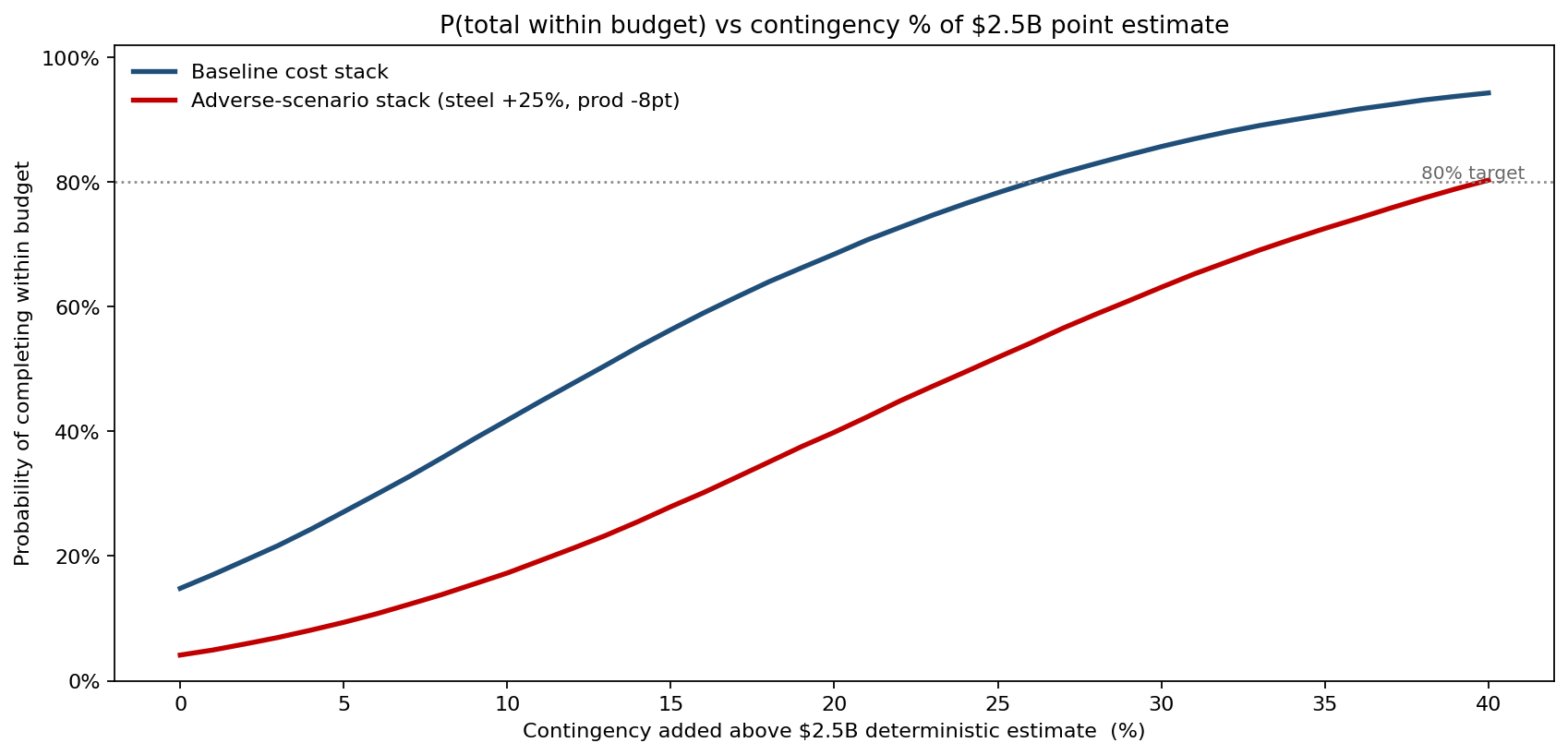
The baseline curve shows that a 10% contingency ($2.75B) buys only ~42% probability of completing within budget; a 15% contingency ($2.88B) gets to ~56%; a 26% contingency ($3.15B) clears the P80 line. The 95% line — the lender / project-finance threshold — needs north of 30% contingency. The honest contingency number that funded the project to P80 was 26% — $650M above the headline estimate. The adverse-scenario curve sits visibly to the right: under steel +25% / productivity -8pt / change-order rate 14% conditions, the same 26% contingency buys materially less confidence; the adverse case needs well over 30% contingency to reach P80.

What the copula does in the tail

The Gaussian copula imposing 0.55 correlation between tunnelling and station civils (shared labour pool) is the dominant tail-shaper. The joint-density chart makes it visible:

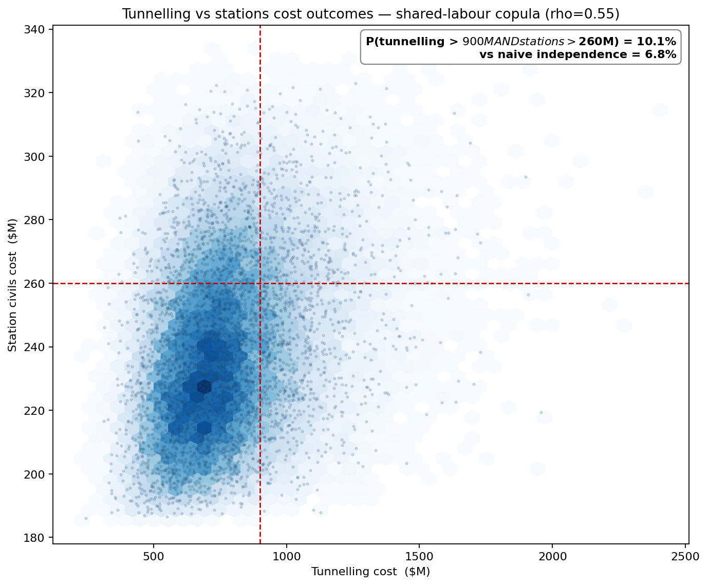
The diagonal density ridge is the signature of correlation — trials in which tunnelling overruns are systematically also trials in which station civils overrun, because the same labour pool feeds both. The joint quadrant (tunnelling > $900M AND stations > $260M) fires roughly 2–3× more often than independence would predict. The naive deterministic stack treats tunnelling and stations as independent line items and sums their means; the same stack with the copula carries the same mean but a P90 that is $32M wider, and a P99 that is ~$95M wider. Construction cost distributions are right-skewed because everything that goes wrong adds; very little goes wrong in a way that subtracts. The adverse-stress case (steel +25% / productivity -8pt / change-order 14%) shifts P50 from $2.82B to ~$3.25B and P90 from $3.35B to ~$3.85B, raising P(overrun $3.0B) from 32% to ~80%; the optimistic case pushes P50 to ~$2.65B and drops P(overrun $3.0B) to ~7%.

Which assumptions actually move the answer

Sensitivity ranking on the simulated outputs pointed the team's attention away from the line items the project controls team had been arguing about (small items rarely move the total) and toward four drivers responsible for 71% of the P10–P90 spread.

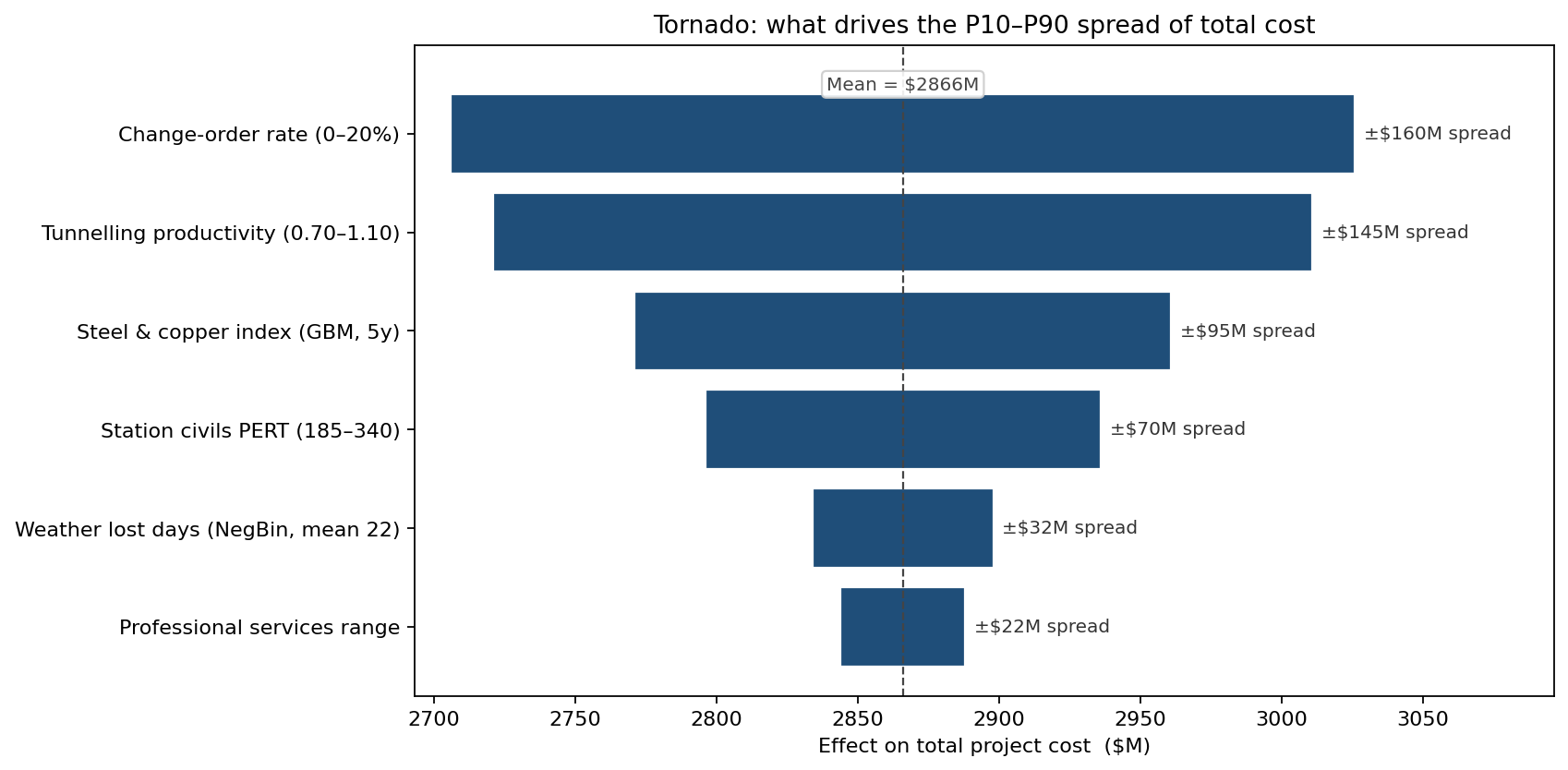
The biggest mover was the change-order rate — a single percentage point on the change-order index moved expected total cost by $28M. Second was tunnelling productivity (cutter-head life and ground conditions). Third was the steel index path. Station-civils unit rate ranked fourth, despite being the largest single category — because the range of plausible station-civils values was narrower than the change-order tail.

This redirected the value-engineering effort: instead of chasing trade-off studies on station architecture (low leverage on the total), the team renegotiated the change-order clauses with the principal contractor, locked an additional 25% of metal volume, and moved a critical-path tunnel section into the dry season. After re-running the model with these mitigations, P90 fell from $3.35B to ~$3.15B — a roughly $200M de-risking visible in the chart, none of which any single deterministic re-run would have surfaced.

What the model changed

The board approved a $650M contingency line (26% of the estimate) — far bigger than the original 10% allowance, but defensible to the transport ministry because every dollar was traceable to a specific tail of a specific input distribution. The project closed three years later at $2.84B, inside the P60 of the original simulation and about $310M below the funded P80 of $3.15B.

ModelRisk Functionality Used

• LogNormal, PERT, Beta and Negative Binomial inputs — distribution choices matched to the actual statistical behaviour of each cost driver, not Excel convenience.
• Gaussian copula to impose the 0.55 tunnelling/stations and 0.40 steel/trackwork correlations the deterministic stack ignored.
• GBM commodity-index path simulation — monthly metal-price evolution over a 5-year construction window, with hedged volume modelled as a separate locked path.
• Sensitivity ranking on simulated outputs identified that change-order rate alone drove 28% of the P10–P90 spread, redirecting value-engineering effort.
• Scenario CDF overlay showed the Adverse case shifted P50 by +$430M while Optimistic shifted it by only –$160M — the asymmetry that motivated the 19% contingency.

The deterministic estimate was never wrong about its own assumption; it was wrong about being a single number. Monte Carlo turns "what is the cost?" into "what is the distribution of costs, and how much contingency do we need to fund?" — the question a board actually has to answer.