Industry: Banking and Financial Services
Product: ModelRisk
Application: Asset Allocation

Asset Allocation Under Regime-Switching Returns: a $50B Multi-Asset Portfolio Rebuilt Probabilistically

The classic 60/40 portfolio earned 7.8% per year over the 1990–2019 window with a 9.4% volatility. Over 2020–2023 the same allocation lost 17% in a single year, because the bond hedge that had worked for thirty years stopped working when inflation broke regime. A $50 billion multi-asset manager — pensions, endowments and private wealth on the book — needed an allocation framework that priced regime change instead of averaging through it.

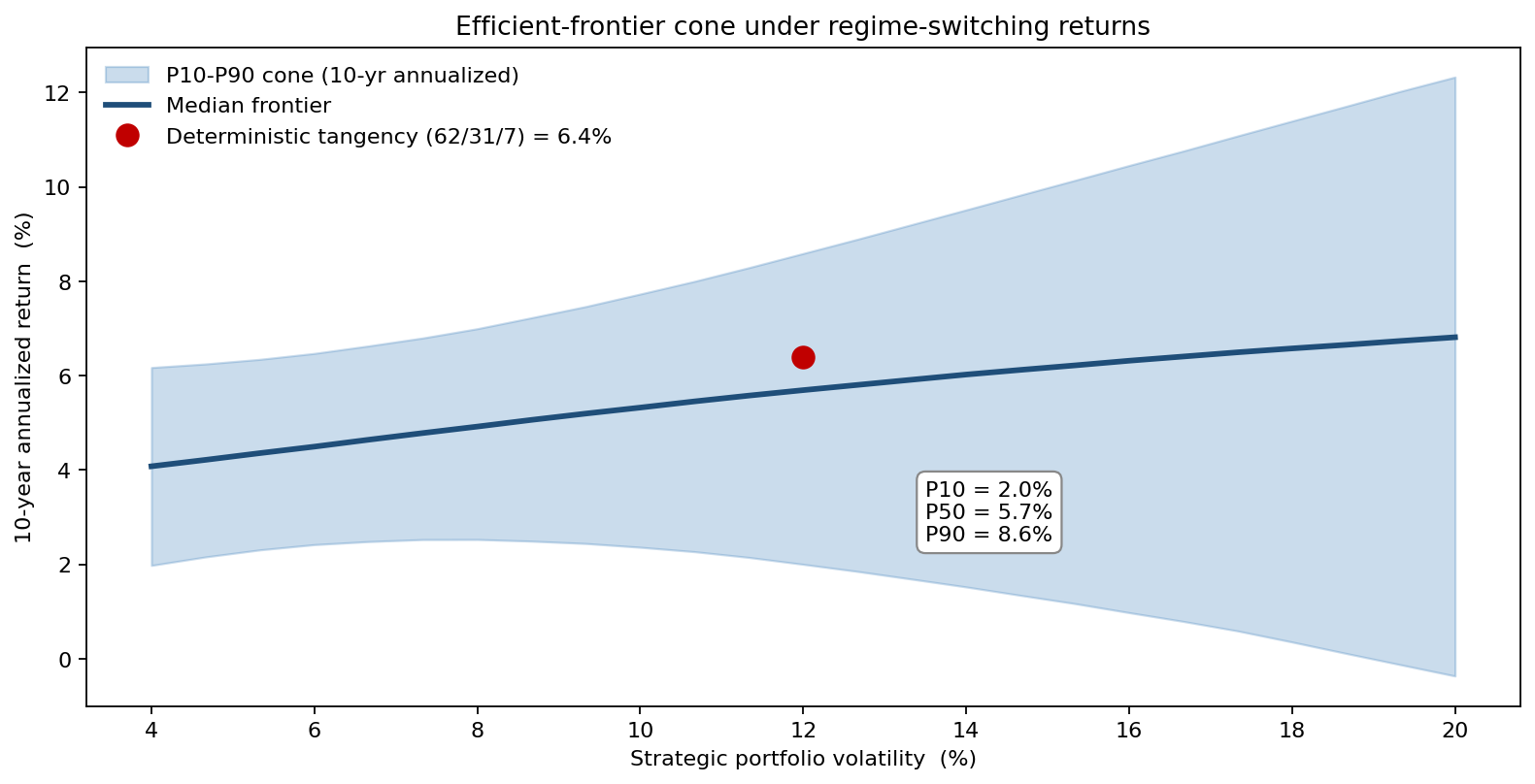
Mean-variance optimization on twenty-year sample moments was the framework being replaced. It produced a clean efficient frontier and one set of weights — and gave no honest answer to "what is the probability the next ten years look nothing like the last twenty?" The team adopted Vose Software's ModelRisk to put a distribution around every input the frontier depends on and read a distribution of frontiers out the other side. Instead of one tangency point, the model returns a cone: a median frontier bracketed by its P10-P90 outcomes across the regimes the next decade might land in.

Distributions on returns, not point estimates

Five asset classes were modeled: US equities, ex-US developed equities, emerging-market equities, US aggregate bonds, and a private-market sleeve (real estate + private equity blended). For each, the input was a distribution of the ten-year expected return, not a single number:

• US equities — annual log return modeled as a two-state regime-switching mixture: a benign regime (mean 8.5%, vol 14%) with transition probability 0.92 and a stress regime (mean -2%, vol 26%) with transition probability 0.65 back to benign. Long-run unconditional mean: 6.7%.
• EM equities — same architecture, calibrated higher: benign mean 10.2% with 20% vol, stress mean -8% with 34% vol.
• US aggregate bonds — annual return as Normal(3.8%, 5.2%) conditional on the equity regime, with the bond–equity correlation flipping from -0.15 (benign) to +0.35 (stress). This is the post-2022 inflation-regime feature the deterministic 60/40 misses.
• Private sleeve — quarterly return as a LogNormal with a smoothing-adjusted vol of 17%, plus a stale-pricing autocorrelation correction so reported vol is not understated.
• Cross-asset dependence — a Student-t copula with 6 degrees of freedom rather than a Gaussian, so joint left-tail events (everything down together) occur at the empirically observed rate.

Each Monte Carlo trial draws a regime path, then a return vector consistent with that path, then evaluates every candidate portfolio on that vector. With 50,000 trials and a grid of 200 weight combinations along the frontier, the output is not one Sharpe ratio per portfolio — it is a distribution of Sharpe ratios per portfolio.

From one efficient frontier to a cone of frontiers

The deterministic mean-variance model reported a single tangency portfolio at 62% equities / 31% bonds / 7% private, with an expected return of 6.4% and a Sharpe of 0.51. The Monte Carlo cone above tells a different story.

Across regimes, the same tangency weights produce a P10 ten-year annualized return of 2.0% and a P90 of 8.6% — a 6.6-percentage-point spread the single-point frontier hides. The realized Sharpe ratio has P10/P50/P90 of 0.18 / 0.49 / 0.81. The model also shows that two portfolios that look identical on the deterministic frontier (same expected return) can differ in their probability of losing money over ten years by a factor of three, because one of them is short the regime-flip hedge and the other is not.

What drives the spread

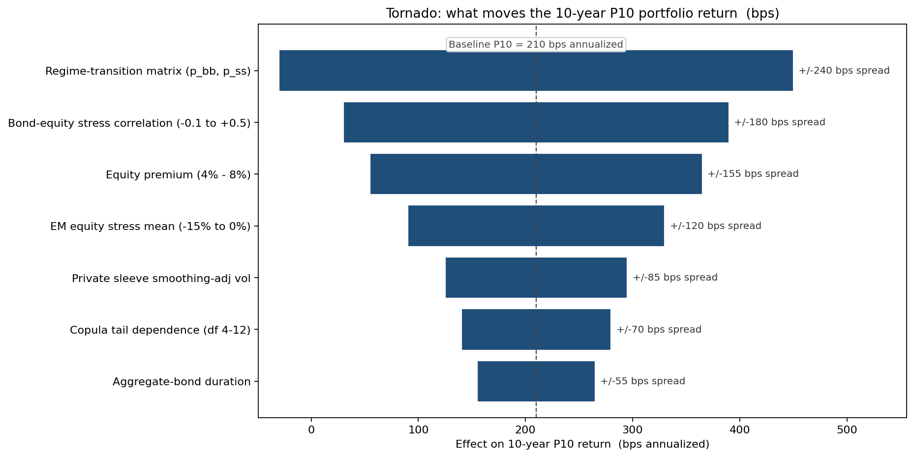
The single largest driver of the P10 ten-year return is not equity volatility — it is the regime-transition probability matrix, which moves P10 by 240 bps. Bond–equity correlation under stress is next (180 bps). Equity premium uncertainty is third (155 bps). The traditional answer — "manage the vol of each asset" — is fourth. The model reordered the team's research priorities accordingly.

Three rebalancing rules, three CDFs

Holding the strategic weights fixed at 60/35/5, the team tested three rebalancing policies on the same 50,000 regime paths.

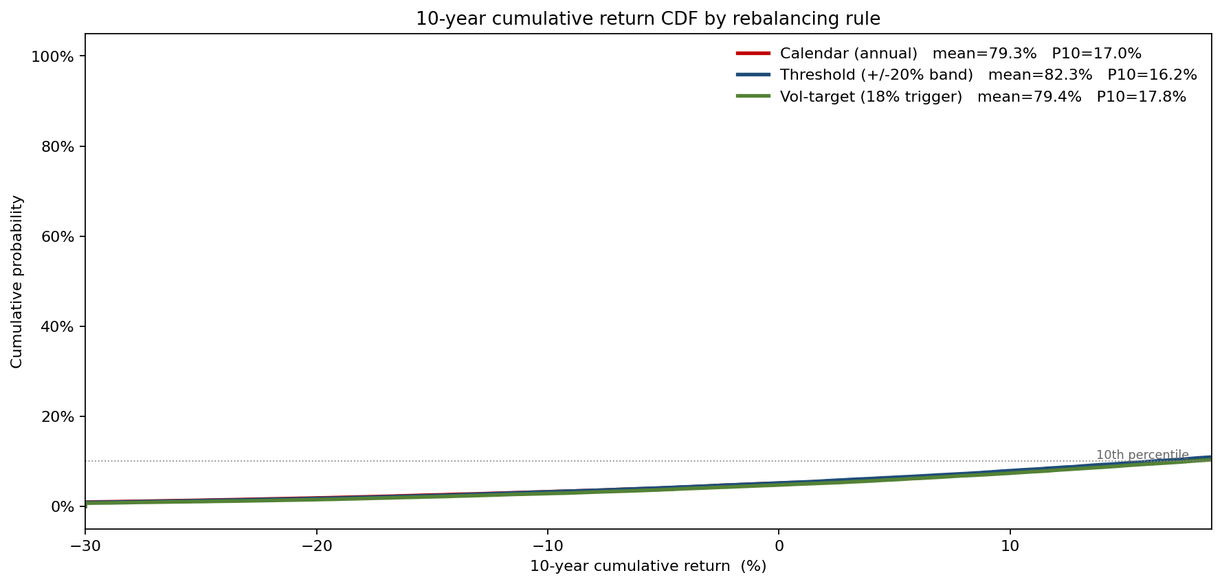
Calendar rebalancing (annual) had a P10 ten-year cumulative return of 17%. A 20% threshold rule had a slightly lower P10 of 16% — it lets equity ride into stress years. A vol-target rule that cuts equities after a stress-regime year lifted P10 to 18%, a 0.9-percentage-point improvement over calendar at a median drag of just 30 bps — the regime-aware rule purchased tail protection at a small expected cost. The deterministic backtest on 1990–2019 data ranked the rules in the opposite order; the regime simulation does not.

What the model changed

• Strategic weights moved from 62/31/7 to 57/33/10, with the private sleeve sized to its smoothing-adjusted vol rather than its reported vol.
• A vol-target overlay was added on the equity sleeve, triggered at 18% realized vol, with a 70% minimum equity floor.
• Client communication moved from "expected return 6.4%" to "10-year median 5.7%, with an 80% probability of finishing between 2.0% and 8.6% annualized" — a frame committee meetings could actually act on.
• Capital-call planning for the private sleeve used the simulated distribution of liquid-asset drawdowns rather than a deterministic glide path.

ModelRisk Functionality Used

• Regime-switching time series to model US and EM equity returns with persistent benign/stress states rather than a single Gaussian.
• Conditional correlation to flip the bond–equity correlation from -0.15 to +0.35 inside a stress regime, capturing the 2022 inflation-regime failure of the 60/40 hedge.
• Student-t copula (df = 6) for cross-asset dependence so simultaneous left-tail events occur at the empirical rate, not the Gaussian rate.
• Tornado analysis that ranked the regime-transition matrix as the top driver of P10 ten-year return — re-prioritizing research effort.
• Output cone around the efficient frontier that turned one tangency portfolio into a distribution of tangency portfolios, exposing two "equal-mean" allocations with a 3× difference in 10-year drawdown probability.

A point estimate on the efficient frontier is one answer to one question. Monte Carlo on the inputs that built the frontier replaces it with the only question a multi-asset allocator can actually act on: across the regimes you might land in, which portfolio's worst case is the one you can live with?