Industry: Agriculture and Food Supply Chain
Product: ModelRisk
Application: Agricultural Economics

The Spreadsheet Said a 2.76M Margin. One Season in Ten It Loses Money.

A 4,000-hectare grain enterprise built its season budget the way every farm office does: take the agronomist's best-guess yield of 8.5 t/ha, multiply by the expected farm-gate price of 210 per tonne, subtract a known cost base, and read off a net margin of 2.76M. It is a perfectly arithmetic answer to the wrong question. The number the bank and the board actually need is not what is the expected margin but how often does this enterprise lose money, and how badly — and that lives in the shape of the distribution, not its centre.

Re-run the same enterprise as a Monte Carlo simulation, with price and yield each carried as a distribution and — crucially — correlated, and the picture sharpens. The mean margin settles at 2.62M, close to the point estimate, but there is a 10% chance of a loss-making season, the P10 margin sits right on the break-even line, and the P5 outcome is a 0.76M loss. The same model also reveals something the point estimate could never show: because low yields and high prices arrive together, the enterprise is far less risky than a naive price-times-yield calculation would suggest.

The natural hedge the point estimate throws away

The single most important fact about farm revenue is that price and yield are negatively correlated. A regional drought cuts every grower's harvest at once, the commodity goes scarce, and the price rises; a bumper season floods the market and the price falls. The two factors partially cancel inside the revenue line Revenue = Price x Yield, so revenue is materially less volatile than either price or yield alone.

This is not a coefficient bolted on after the fact. The model drives both factors from one shared seasonal weather draw: a good growing season pushes yield up (a Beta-shaped season yield, mean 8.5 t/ha, P10–P90 of 5.2 to 11.9 t/ha) and simultaneously pushes price down, while an independent global-market term (a LogNormal carrying macro, FX and trade-policy noise, P10–P90 of 152 to 279 per tonne) does not cancel against this farm's yield. The resulting empirical price-yield correlation is -0.40 — the natural hedge, made explicit.

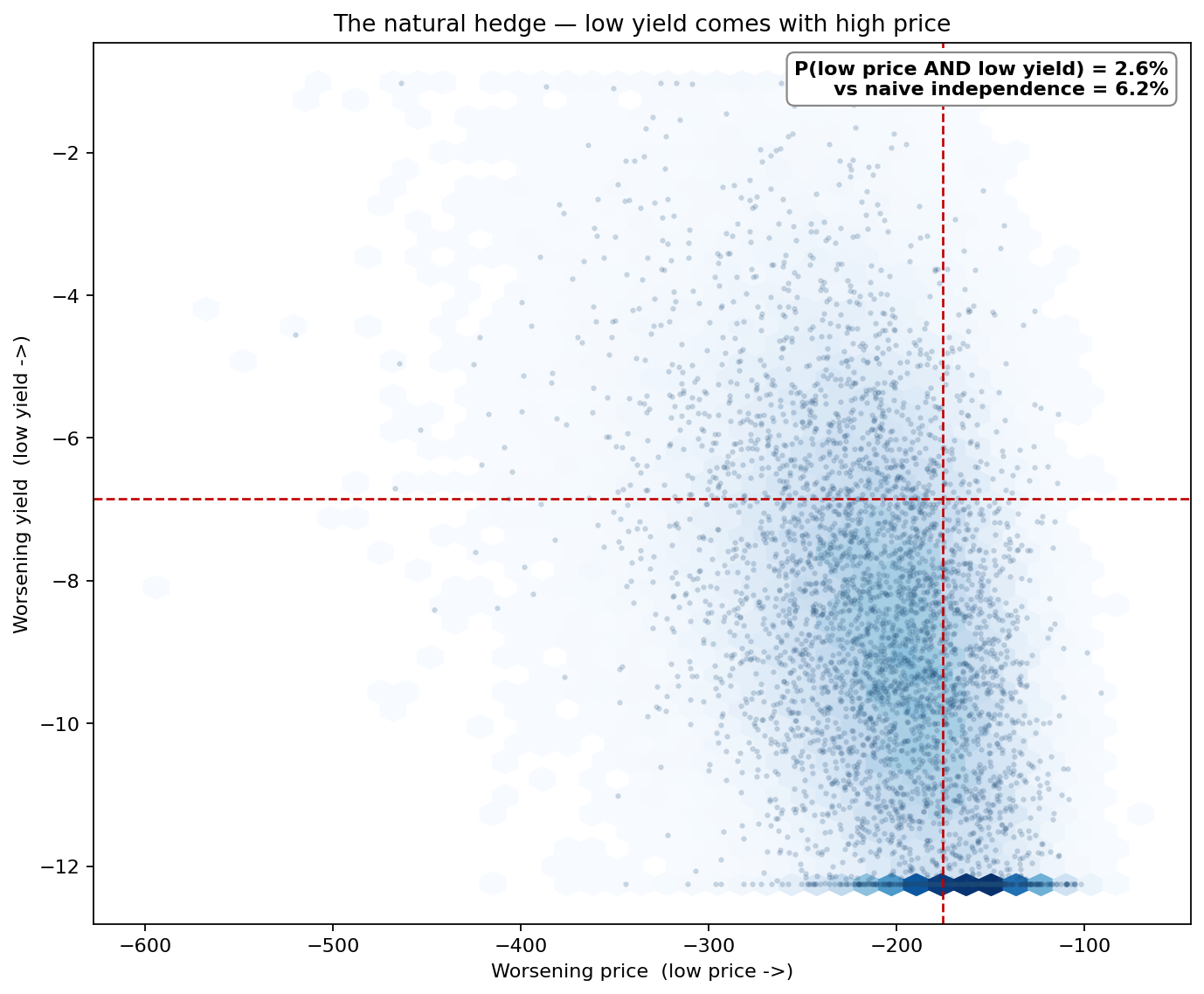
The joint density makes the hedge visible. The dangerous corner for revenue — low price AND low yield at the same time — occurs in only 2.6% of seasons, against the 6.2% a naive independence assumption would predict. The cloud tilts: the bottom-left revenue-collapse quadrant is starved of points precisely because the weather factor that empties the silo also empties the market.

Why a point estimate fails here

A single margin figure hides two things at once. First, it hides the loss tail: the 2.76M point estimate sits comfortably in the black, but the distribution it summarises crosses zero one season in ten. Second — and this is the subtler failure — a planner who does try to stochastically stress price and yield, but treats them as independent, overstates the enterprise's risk.

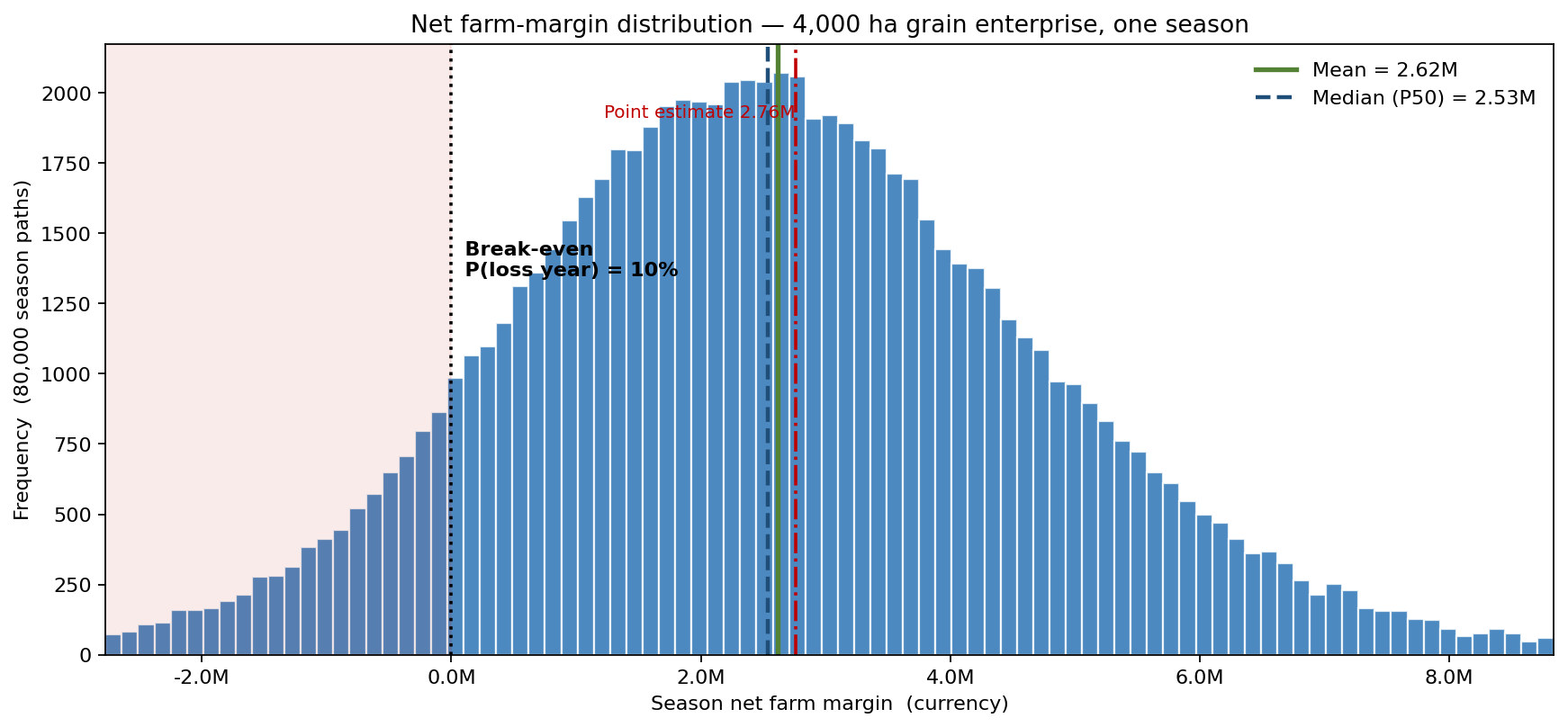
The headline distribution puts numbers on it. The mean margin is 2.62M and the median 2.53M, against the deterministic 2.76M. The break-even line is crossed with probability 10% — the loss-year frequency the spreadsheet was silent on. The point estimate is not wildly optimistic on the mean; it is simply blind to the lower tail that determines whether the enterprise can service its debt in a bad year.

What the hedge is worth

To value the hedge, the same simulation was run twice: once with the correlated price and yield, and once with the price stream shuffled so the two are independent but keep identical marginals.

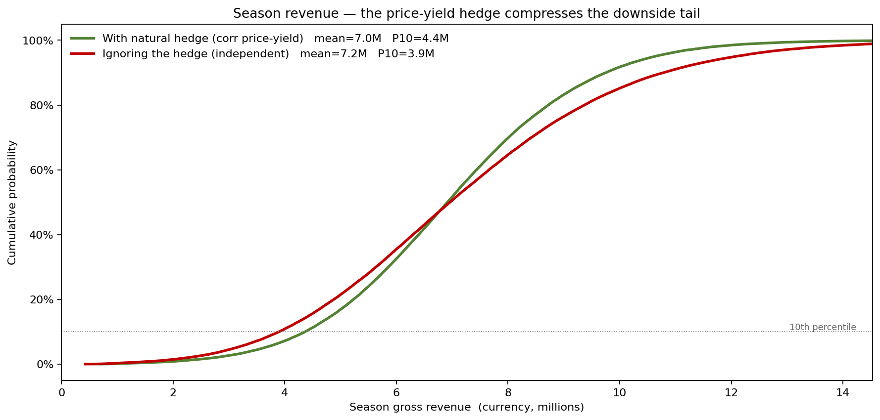
The hedge compresses exactly the part of the distribution the farm finances against. Revenue's coefficient of variation falls from 38.1% under the independence assumption to 30.6% with the correlation in place, and the P10 (worst-decile) revenue rises from 3.90M to 4.36M — half a million of downside protection the farm gets for free from the structure of agricultural markets. Ignore the hedge and the model would have reported a 14.4% loss-year probability instead of the true 10.2%, over-stating tail risk by 40% and potentially triggering hedging the farm did not need.

What actually moves the margin

With four uncertain inputs, the next question is which ones the answer depends on.

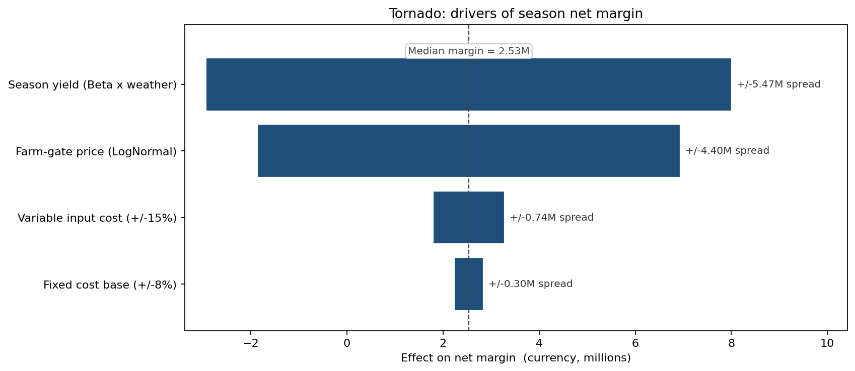
The tornado ranks them on their P10–P90 swing of net margin. Season yield is the dominant driver at +/-2.74M, just ahead of farm-gate price at +/-2.20M; the two input-cost levers are an order of magnitude smaller (variable input cost +/-0.37M, the fixed-cost base +/-0.15M). The message is operational: chasing a few percent off fertiliser spend is rearranging deckchairs next to the yield-and-price exposure, and that exposure is best managed through the revenue line — agronomy and marketing — not the cost line.

From insight to action

The enterprise acted on the distribution, not the mean:

1. Revenue insurance sized to the residual tail. A policy guaranteeing 85% of expected revenue carries a fair premium of 0.45M and removes the loss-year probability entirely — from 10.2% to 0%. With the hedge already doing most of the work, insurance is a cheap top-up rather than the first line of defence.
2. Forward sales sized against P10, not the mean. Knowing the P10 yield is 5.2 t/ha, the enterprise pre-sells a tonnage it can deliver in nine seasons out of ten rather than committing to its best guess.
3. No over-hedging of price. Because the natural hedge already trims revenue volatility by a fifth, the board declined an expensive price-only hedging programme that an independence-based model would have justified.

ModelRisk functionality used

• Monte Carlo simulation propagating a Beta-shaped yield and a LogNormal price through Revenue = Price x Yield - Cost across 80,000 season paths to produce the full net-margin distribution.
• Correlation via a shared driver — a single seasonal weather factor loading yield and price in opposite directions, reproducing the empirical -0.40 price-yield correlation rather than assuming independence.
• Scenario comparison running the model with correlated and independent price-yield streams to quantify the hedge (revenue CV 30.6% vs 38.1%).
• Tornado sensitivity ranking the four margin drivers, isolating yield (+/-2.74M) and price (+/-2.20M) as the pair that matters.
• Output visualisation — margin histogram, price-yield joint density, revenue CDFs and tornado — to make the hedge legible to a board reasoning about debt service.

Monte Carlo turns farm economics from "what is the expected margin?" into "how often does this enterprise lose money, and how much of that risk does the market already hedge for free?" — and on this farm the answer was a 10% loss-year probability and a fifth of revenue volatility quietly cancelled by the price-yield correlation.