Discounted cash flow modeling

First have a look at the following diagram:

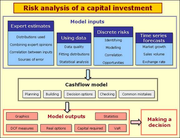
A typical discounted cashflow model for a potential investment makes forecasts of costs and revenues over the life of the project and discounts those revenues back to a present value. Most analysts start with a 'base case' model and add uncertainty to the important elements of the model. Happily, the mathematics involved in adding risk to these types of models is quite simple. In this topic we assume that you can build a base case cashflow model that will look something like the example model shown below. We will then focus on the input modelling elements and some financial outputs.

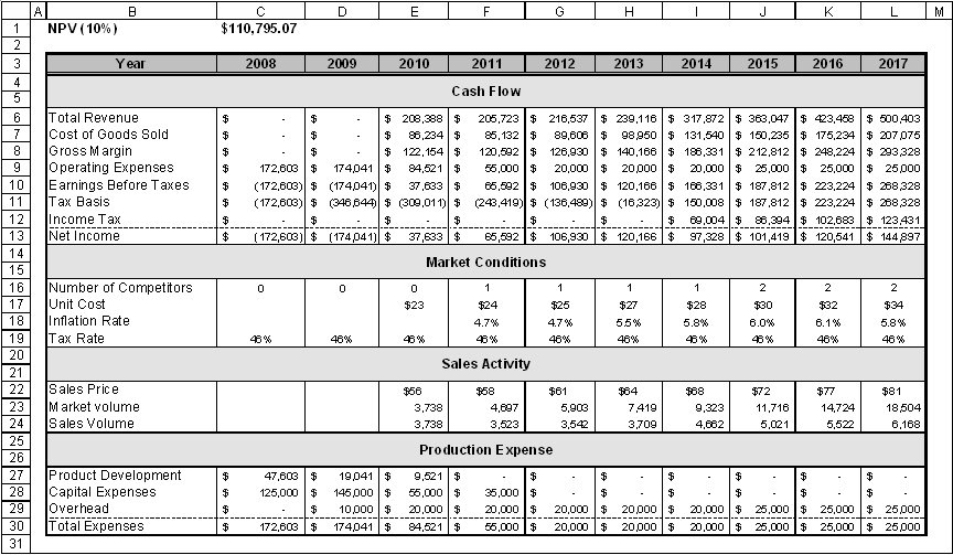
Example model NPV of a capital investment (tab Static model) - a typical, if somewhat reduced, cash flow model.

There are a number of relevant topics that are covered in other parts of this help file. Please make sure you have a good understanding of these first:

Modeling expert opinion

In capital investment models we rely a great deal on expert judgement to estimate variables like costs, time to market, sales volumes, discount levels

Fitting distributions to data

We don't usually have a great deal of historic data to work with in capital investment projects because the investment is new. I have worked with a very successful retail company that investigates levels of pedestrian traffic at different locations in a town where it is considering locating a new outlet. It has excellent regional data on how that traffic converts to till receipts. That is quite typical of the type of data one might have for a cashflow analysis and we will go through such a model later in this topic. Hydrocarbon and mineral exploration will generally have improving levels of data about the reserves, but have specialised methods for statistically analyzing (e.g. Krieging) their data, so I won't consider them further here.

Modeling correlation

Simple forms of correlation modelling - recognizing that two or more variables are likely to be linked in some way - are very important in cashflow models.

Time series

The time series topics deal with many different technical time series models. GBM, seasonal and autoregressive models are useful for modelling inflation, exchange and interest rates over time in a cashflow model. Lead indicators can help predict market size a short time into the future. In this topic consider variables like demand for products and sales volumes which are generally built on a more intuitive basis.

Common errors in risk modeling

Risk analysis cashflow models are not generally that technically complicated, but our reviews show that the types of errors described under Common errors in risk modeling appear very frequently, so we encourage you to read that section carefully. The rest of this topic offers some ideas on model building that are very applicable to cashflow models.

Useful time series models of sales and market size

Effect of an intervention at some uncertain point in time

Time series variables are often affected by single identifiable 'shocks', like elections, changes to a law, introduction of a competitor, start or finish of a war, a scandal, etc. The modelling of the occurrence of a shock and its effects may need to take into account several elements:

When the shock may occur (this could be random);
Whether this changes the probability or impact of other possible shocks;
The effect of the shock: magnitude and duration

Consider the following problem: People are purchasing your product at a current rate of 88/month, and the rate appears to be increasing by 1.3 sales/month with each month. However, we are 80% sure that a competitor is going to enter the market and will do so between 20 and 50 months from now. If the competitor enters the market they will take about 30% of your sales. Forecast the number of sales there will be for the next 100 months.

Possible pathways generated by the model depending on whether the competitor enters the market

The model for this problem is shown in the figure above . The Bernoulli variable returns a 1 with 80% probability, otherwise a 0. It is used as a 'flag', the 1 representing a competitor entry, the 0 representing no competitor. Other cells use conditional logic to adapt to the scenario.

The StepUniform generates integer values between 20 and 50, and cell E4 returns the month 1000 if the competitor does not enter the market i.e. a time beyond the modelled period. It is a good idea if you use this type of technique to make such a number very far from the range of the modelled period in case someone decided to extend the period analyzed. A Poisson distribution is used to model the number of sales reflecting that the sales are independent of each other and randomly distributed in time. The nice thing about a Poisson distribution is that it takes just one parameter - its mean, so you don't have to think about variation about that mean separately (e.g. determine a standard deviation).

Example model Poisson_sales_with_competitor - Poisson sales affected by the possible entry of a competitor

Distributing market share

When competitors enter an established market they have to establish the reputation of their product and fight for market share with others that are already established. This takes time, so it is more realistic to model a gradual loss of market share to competitors.

Consider the following problem: Market volume for your product is expected to grow each year by (10%, 20%, 40%) beginning next year at (2500, 3000, 5000) up to a maximum of 20,000 units. You expect one competitor to emerge as soon as the market volume reaches 3,500 units in the previous year. A second would appear at 8,500 units. Your competitors' shares of the market would grow linearly until you all have equal market share after three years. Model the sales you will make.

Example model New_competitors - sales where the total market is divided with new entry competitors

The figure above shows the model. It is mostly self-explanatory. The interesting component lies in Cells F10:L10 which divides the forecast market for your product among the average of the number of competitors over the last three years and yourself (the '1' in the equation). Averaging over three years is a neat way of allocating an emerging competitor 1/3 of your market strength in the first year, 2/3 in the second and equal strength from the third year on - meaning that they will then sell as many units as you. What is so helpful about this little trick is that it automatically takes into account each new competitor and when they entered the market, which is rather difficult to do otherwise. Note that we need three zeros in cells C8:E8 to initialise the model.

Reduced sales over time to a finite market

Some products are essentially a once in a lifetime purchase, e.g. a life insurance, big flat screen TV, a new guttering system and a pet identification chip. If we are initially quite successful in selling the product into the potential market, the remaining market size decreases although this can be compensated to some degree by new potential consumers. Consider the following problem: There are currently PERT(50000,55000,60000) possible purchasers of your product. Each year there will be about a 10% turnover (meaning 10% more possible purchasers will appear). The probability that you will sell to any particular purchaser in a year is PERT(10%,20%,35%). Forecast sales for the next 10 years.

Example model Finite_market - forecasting sales over time to a finite market

The figure above shows the model for this problem. Note that C8:C16 is subtracting sales already made from the previous year's market size but also adding in a regenerated market element. The Binomial distribution then converts the current market size to sales. In the particular scenario shown in the figure the probability of selling is high (26%) so sales start off high and drop off quickly since the regeneration rate is so much lower (10%). Note that some Monte Carlo software cannot handle large numbers of trials in their Binomial distribution in which case you will need to use a Poisson or Normal approximation.

Growth of sales over time up to a maximum as a function of marketing effort

Sometimes we might find it easier to estimate what our annual sales will be when stabilized, but be unsure of how quickly we will be able to achieve that stability. In this sort of situation it can be easier to model a theoretical maximum sales and match it to some ramping function. A typical form of such a ramping function r(t) is:

which will produce a curve that starts at 0 for t = 0 and asymptotically reaches 1 at an infinite value of t, but reaches 0.5 at . Consider the following problem: you expect a final sales rate of PERT(1800,2300,3600) and expect to achieve half that in the next PERT(3.5,4,5) years. Produce a sales forecast for the next 10 years.

The example model below provides a solution:

Example model Sales_with_maximum - forecasting ramping sales to an uncertain theoretical maximum

Summing random variables

Perhaps the most common errors in cashflow modelling occur when one wishes to sum a number of random costs, sales or revenues. For example, imagine that you expect to have Lognormal(100 000, 25 000) customers enter your store per year and they will spend $Lognormal(55, 12) each - how would you estimate the total revenue? People generally write something like:

= ROUND(Lognormal(100 000, 25 000),0) * $Lognormal(55, 12) (equation 1)

using the ROUND function in Excel to recognise that the number of people must be discrete. But let's think what happens when the software starts simulating. It will pick a random value from each distribution and multiply them together. Picking a reasonably high till receipt, the probability that a random customer will spend more than $70, for example, is:

=1-VoseLognormalProb(70,55,12,1) = 0.11%

The probability that two people will do the same is 11% * 11% = 1.2%, and the probability that thousands of people will spend that much is infinitesimally small. However, Equation 1 will assign a 11% probability that all customers will spend over $70 no matter how many there are. The equation is wrong because it should have summed ROUND(Lognormal(100 000, 25 000),0) separate Lognormal(55, 12) distributions. That's a big, slow model so we use a variety of techniques to shortcut to the answer, which is the topic of aggregate modeling.

Summing variable margins on variable revenues

A common situation is that we have a large random number of revenue items that follow the same probability distribution but which are independent of each other, and we have independent profit margins that follow another distribution that must be applied to each revenue item. This type of model quickly becomes extremely cumbersome to model because for each revenue item we need two distributions: one for revenue and another for the profit margin and we may have many types of large numbers of revenue items. It is such a common problem that we designed a function in ModelRisk to handle this, allowing you to keep the model to a manageable size, speeding up simulation time, and making the model far simpler to review. Perhaps most importantly, it allows you to avoid a lot of conditional logic that is easy to get wrong. Consider the following problem: a capital venture company is considering investing in a company that makes TV shows. They expect to make PERT(28,32,39) pilots next year which will generate revenues of $PERT(120,150,250)k each independently and from which the profit margin is PERT(1%,5%,12%). There is a 30% chance that each pilot is made into a TV series run in that country running for Discrete({1,2,3,4,5},{0.4,0.25,0.2,0.1,0.05}) series, where each season of each series generates $PERT(120,150,250)k with margins of PERT(15%,25%,45%). There is a 20% chance that these local series would be sold to the US generating $PERT(240,255,1350) per season sold of which the profit margin is PERT(65%,70%,85%). What is the total profit generated from next year's pilots?

Example model TV_series_profits - forecasting profits from a TV series

The problem is not technically difficult but the scale of the modelling explodes very quickly. We worked on the model for a real investment of this type and it had many more layers: pilots in several countries, merchandising of various types, repeats, etc. and it took a lot of effort to manage. The figure shows how using objects for modeling allows us a surprisingly succinct model: rows 2 to 12 are the input data, rows 14 to 16 are the actual calculations.

There are a few things to point out. In Cell F2, ½ is subtracted and added to the minimum and maximum estimates respectively of the number of pilots to give a more realistic chance of their occurrence after rounding. Distributions are input as ModelRisk objects in cells F3, F4, F6, F7, F8, F10 and F11 because we want to use these distributions many times. Cell C16 and elsewhere uses the VoseSumProduct function to add together revenue * margin for each pilot where the revenue and margin distributions are defined by the distribution Objects in Cells F3 and F4 respectively. Cell F14 simulates the number of pilots that made it to become series, from which the model determines how many of those become series also sold into the US in Cell E14, the difference being the number of pilots that only became local series in Cell D14. Setting up the logic this ways ensures that we have a consistent model: the local only and US & local series always add up to the total series produced. Cells D15 and E15 use the VoseAggregateMC(x, y) function to simulate the sum of x random variables all taking the same distribution y defined as an Object.

Financial measures in risk analysis

The two main measures of profitability in DCF models are net present value (NPV) and internal rate of return (IRR). The two main measures of financial exposure are VAR and expected shortfall. Their pros and cons are discussed below.

Net Present Value

Net Present Value (NPV) attempts to determine the present value of a series of cashflows from a project that stretches out into the future. This present value is a measure of how much the company is gaining at today's money by undertaking the project: in other words, how much more the company itself will be worth by accepting the project.

An NPV calculation discounts future cashflows at a specified discount rate r that takes account of:

the time value of money (e.g. if inflation is running at 4%, £1.04 in a year's time is only worth £1.00 today);
the interest that could have been earned over inflation by investing instead in a guaranteed investment;
the extra return that is required over (1) and (2) to compensate for the degree of risk that is being accepted in this project;

Parts (1) and (2) are combined to produce the risk free interest rate, r_f. This is typically determined as the interest paid by guaranteed fixed payment investments like government bonds with a term roughly equivalent to the duration of the project.

The extra interest r^* over r_f needed for (3) is determined by looking at the uncertainty of the project. In risk analysis models, this uncertainty is represented by the spread of the distributions of cashflow for each period. The sum of r^* and r_f is called the risk-adjusted discount rate r.

The most commonly used calculation for the NPV of a cashflow series over n periods is as follows:

where are the expected (i.e. average) values of the cashflows in each period and r is the risk-adjusted discount rate.

NPV calculations performed in a risk analysis spreadsheet model are usually presented as a distribution of NPVs because the cashflow values selected in the NPV calculations are their distributions rather than their expected values. Theoretically, this is incorrect. Since an NPV is the net present value, it can have no uncertainty. It is the amount of money that the company values the project at today. The problem is that we have double counted our risk by first discounting at the risk-adjusted discounted rate r and then showing the NPV as a distribution (i.e. it is uncertain).

Two theoretically correct methods for calculating an NPV in risk analysis are discussed below, along with a more practical, but strictly speaking incorrect, alternative:

Theoretical approach 1: Discount the cashflow distributions at the risk free rate.

This produces a distribution of NPVs at r_f and ensures that the risk is not double-counted. However, such a distribution is not at all easy to interpret since decision makers will almost certainly never have dealt with risk free rate NPVs and therefore have nothing to compare the model output against.

Theoretical approach 2: Discount the expected value of each cashflow at the risk-adjusted discount rate.

This is the application of the above formula. It results in a single figure for the NPV of the project. A risk analysis is run to determine the expected value and spread of the cashflows in each period. The discount rate is usually determined by comparing the riskiness associated with the project's cashflows against the riskiness of other projects in the company's portfolio. The company can then assign a discount rate above or below its usual discount rate depending on whether the project being analyzedexhibits more or less risk than the average. Some companies determine a range of discount rates (three or so) to be used against projects of different riskiness.

The major problems of this method are that it assumes the cashflow distributions are symmetric and that no correlation exists between cashflows. Distributions of costs and returns almost always exhibit some form of asymmetry and in a typical investment project there is also always some form of correlation between cashflow periods: for example, sales in one period will be affected by previous sales, a capital injection in one period often means that it doesn't occur in the next one (e.g. expansion of a factory) or the model may include a time series forecast of prices, production rates or sales volume that are autocorrelated. If there is a strong positive correlation between cashflows, this method will overestimate the NPV. Conversely, a strong negative correlation between cashflows will result in the NPV being underestimated. The correlation between cashflows may take any number of, often complex, forms. Financial theory does not offer a practical method for adjusting the NPV to take account of these correlations.

In practice, it is easier to apply the risk-adjusted discount rate r to the cashflow distributions to produce a distribution of NPVs. This method incorporates correlation between distributions automatically and enables the decision maker to compare directly with past NPV analyses.

As I have already explained, the problem associated with this technique is that it will double count the risk: firstly in the discount rate and then by representing the NPV as a distribution. However, if one is aware of this shortfall, the result is very useful in determining the probability of achieving the required discount rate (i.e. the probability of a positive NPV). The actual NPV to quote in a report would be the expected value of the NPV distribution.

Internal Rate of Return

The Internal Rate of Return (IRR) of a project is the discount rate applied to its future cashflows such that it produces a zero NPV. In other words, it is the discount rate that exactly balances the value of all costs and revenues of the project. If the cashflows are uncertain, the IRR will also be uncertain and therefore have a distribution associated with it.

A distribution of the possible IRRs is useful to determine the probability of achieving any specific discount rate and this can be compared with the probability other projects offer of achieving the target discount rate. It is not recommended that the distribution and associated statistics of possible IRRs be used for comparing projects because of the following properties of IRRs:

· Unlike the NPV calculation, there is no exact formula for calculating the IRR of a cashflow series. Instead, a first guess is usually required, from which the computer will make progressively more accurate estimates until it finds a value that produces an NPV as near to zero as required.

· If the cumulative cashflow position of the project passes through zero more than once, there is more than one valid solution to the IRR inequality. This is not normally a problem with deterministic models because the cumulative cashflow position can easily be monitored and the smallest of any IRR solutions selected. However, a risk analysis model is dynamic, making it difficult to appreciate its exact behaviour. Thus, the cumulative cashflow position may pass through zero and back in some of the risk analysis iterations and not be spotted. This can produce quite inaccurate distributions of possible IRRs. In order to avoid this problem, it may be worth including a couple of lines in your model that calculate the cumulative cashflow position and the number of times it passes through zero. If this is selected as a model output, you will be able to determine whether this is a statistically significant problem and alter the first guess to compensate for it.

· IRRs cannot be calculated for only positive or only negative cashflows. IRRs are therefore not useful for comparing between two purely negative or positive cashflow options, e.g. between hiring or buying a piece of equipment.

· It is difficult to compare distributions of IRR between two options unless the difference is very large. This is because a percentage increase in an IRR at low returns (e.g. from 3% to 4%) is of much greater real value than a percentage increase at high returns (e.g. from 30% to 31%). It is therefore very difficult to compare the value of two projects in terms of the IRR distributions they offer. One project may offer a long right-hand tail that can easily increase the expected IRR but in real value terms this could easily be outweighed by a comparatively small diminishing of the left-hand tail of the other option.

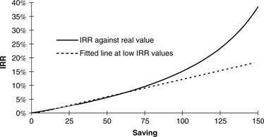
An example of the non-linear relationship between IRR and real (or present) value.